Excel Gurus Gone Wild

Do the IMPOSSIBLE with Microsoft Excel

Bill Jelen

• Publisher: Holy Macro! Books
• Year: 2009
• Print ISBN: 9781932802405
• eBook ISBN: 9781615474011
• Edition: 1
• Topic: Computer Science
• Subtopic: Desktop Applications
• Index: Computer Science

Drawn from actual excel conundrums posted on the author's website, www.mrexcel.com, this high-level resource is designed for people who want to stretch Excel to its limits. Tips for solving 100 incredibly difficult problems are covered in depth and include extracting the first letter of each word in a paragraph, validating URL's, generating random numbers without repeating, and hiding rows if cells are empty. The answers to these and other questions have produced results that have even surprised the Excel development team.

PART 1

FORMULAS

Find the First Non-Blank Value in a Row

Challenge: You want to build a formula to return the first non-blank cell in a row. Perhaps columns B:K reflect data at various points in time. Due to the sampling methodology, certain items are checked infrequently.

Solution: In Figure 1, the formula in A4 is:

Although this formula deals with an array of cells, it ultimately returns a single value, so you do not need to use Ctrl+Shift+Enter when entering this formula.

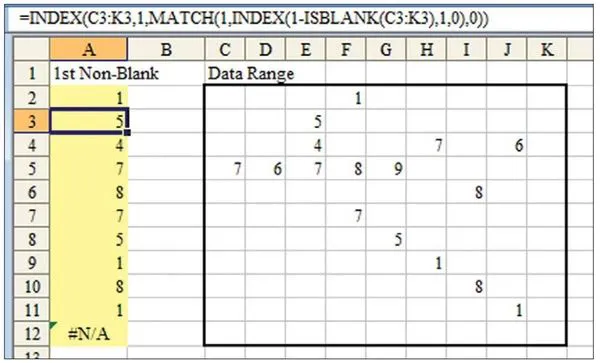
Figure 1. You find the first non-blank cell in each row of C2:K12 and return that value in column A.

Breaking It Down: Let’s start from the inside. The ISBLANK function returns TRUE when a cell is blank and FALSE when a cell is non-blank. Look at the row of data in C4:K4. The ISBLANK(C4:K4) portion of the formula will return:

Notice that this array is subtracted from 1. When you try to use TRUE and FALSE values in a mathematical formula, a TRUE value is treated as a 1, and a FALSE value is treated as a 0. By specifying 1-ISBLANK (C4:K4), you can convert the array of TRUE/FALSE values to 1s and 0s. Each TRUE value in the ISBLANK function changes to a 0. Each FALSE value changes to a 1. Thus, the array becomes:

The formula fragment 1 - I SBLANK (C4 : K4) specifies an array that is 1 row by 9 columns. However, you need Excel to expect an array, and it won’t expect an array based on this formula fragment. Usually, the INDEX function returns a single value, but if you specify 0 for the column parameter, the INDEX function returns an array of values. The fragment INDEX (1-ISBLANK (C4:K4),1,0) asks for row 1 of the previous result to be returned as an array. Here’s the result:

The MATCH function looks for a certain value in a one-dimensional array and returns the relative position of the first found value. =MATCH (1, Array, 0) asks Excel to find the position number in the array that first contains a 1. The MATCH function is the piece of the formula that identifies which column contains the first non-blank cell. When you ask the MATCH function to find the first 1 in the array of 0s and 1s, it returns a 3 to indicate that the first non-blank cell in C4 : K4 occurs in the third cell, or E4:

Formula fragment: MATCH (1, INDEX (1-ISBLANK (C4 : K4), 1, 0), 0)

Sub-result: MATCH (1, {0, 0, 1, 0, 0, 1, 0, 1, 0}, 0)

Result: 3

At this point, you know that the third column of C4 : K4 contains the first non-blank value. From here, it is a simple matter of using an INDEX function to return the value in that non-blank cell. =INDEX (Array, 1, 3 ) returns the value from row 1, column 3 of an array:

Formula fragment: =INDEX (C4 :K4, 1, MATCH (1, INDEX (1-ISBLANK (C4 : K4),1,0),0))

Sub-result: =INDEX (C4 : K4 , 1, 3)

Result: 4

Additional Details: If none of the cells are non-blank, the formula returns an #N/A error.

Alternate Strategy: Subtracting the ISBLANK result from 1 does a good job of converting TRUE/FALSE values to 0s and 1s. You could skip this step, but then you would have to look for FALSE as the first argument of the MATCH function:

Summary: The formula to return the first non-blank cell in a row starts with a simple ISBLANK function. Using INDEX to coax the string of results into an array allows this portion of the formula to be used as the lookup array of the MATCH function.

Source: http://www.mrexcel.com/forum/showthread.php?t=53223

CALCULATE WORKDAYS FOR 5-, 6-, AND 7-DAY WORKWEEKS

Challenge: Calculate how many workdays fall between two dates. Excel’s NETWORKDAYS function does this if you happen to work the five days between Monday and Friday inclusive. This topic will show you how to perform the calculation for a company that works 5, 6, or 7 days a week.

Background: The NETWORKDAYS function calculates the number of workdays between two dates, inclusive of the beginning and ending dates. You specify the earlier date as the first argument, the later date as the second argument, and optionally an array of holidays as the third argument. In Figure 2, cell C3 calculates only 5 workdays because February 16, 2009, is a holiday. This is a cool function, but if you happen to work Monday through Saturday, it will not calculate correctly for you.

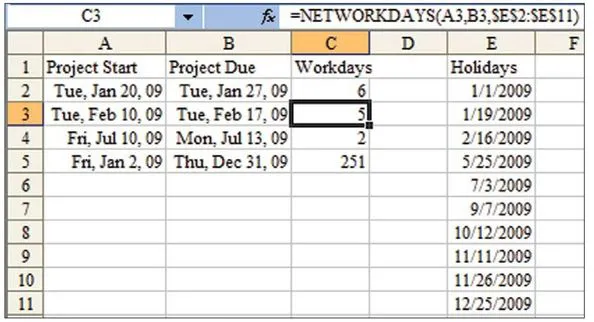
Figure 2. Traditionally, NETWORKDAYS assumes a Monday – through-Friday workweek.

Setup: Define a range named Holidays to refer to the range of holidays.

Solution: The formula in C3 is:

Although this formula deals with an array of cells, it ultimately returns a single value, so you do not need to use Ctrl+Shift+Enter when entering this formula.

Breaking It Down: The formula seeks to check two things. First, it checks whether any of the days within the date r...

Table of contents

• Title Page
• Copyright Page
• ABOUT THE AUTHOR
• ACKNOWLEDGMENTS
• Dedication
• FOREWORD
• Table of Contents
• PART 1 - FORMULAS
• PART 2 - TECHNIQUES
• PART 3 - MACROS
• APPENDIX 1 - ALPHABETICAL FUNCTION REFERENCE
• Also from Bill Jelen - Available at Bookstores Everywhere