PT Symmetry

In Quantum and Classical Physics

Carl M Bender

• Publisher: WSPC (EUROPE)
• Year: 2018
• eBook ISBN:
  9781786345974
• Topic: Sciences physiques
• Subtopic: Physique mathématique et informatique

Originated by the author in 1998, the field of PT (parity-time) symmetry has become an extremely active and exciting area of research. PT-symmetric quantum and classical systems have theoretical, experimental, and commercial applications, and have been the subject of many journal articles, PhD theses, conferences, and symposia. Carl Bender's work has influenced major advances in physics and generations of students.

This book is an accessible entry point to PT symmetry, ideal for students and scientists looking to begin their own research projects in this field.

Contents:

• Preface
• About the Authors
• Acknowledgments
• Introduction to PT Symmetry:
  • Basics of PT Symmetry
  • PT -Symmetric Eigenvalue Problems
  • PT -Symmetric Quantum Mechanics
  • PT -Symmetric Classical Mechanics
  • PT -Symmetric Quantum Field Theory
• Advanced Topics in PT Symmetry:
  • Proof of Reality for Some Simple Examples
  • Exactly Solvable PT -Symmetric Models
  • Kreĭn-Space Theory and PTQM
  • PT -Symmetric Deformations of Nonlinear Integrable Systems
  • PT Symmetry in Optics

Readership: Advanced graduate students and researchers, scientists, mathematicians, and engineers in many fields.PT Symmetry;Non-Hermitian Hamiltonian;Exceptional Points00

Part I

Introduction to PT Symmetry

By Carl M. Bender with Daniel W. Hook

“Numbers have a way of taking a man by the

hand and leading him down the path of reason.”

—PyThagoras

Chapter 1

Basics of PT Symmetry

“We consider it a good principle to explain the
phenomena by the simplest hypothesis possible.”

–PT olemy

This chapter introduces the basic ideas of PT-symmetric systems. It begins with a brief discussion of closed (isolated) and open (non-isolated) systems and explains that PT-symmetric systems are physical configurations that may be viewed as intermediate between open and closed systems. The chapter then presents elementary examples of quantum-mechanical and classical PT-symmetric systems. It demonstrates that the Hamiltonians that describe PT-symmetric systems are complex extensions (deformations) of conventional real Hamiltonians. Finally, this chapter shows that real systems that are unstable may become stable in the more general complex setting. Thus, by deforming real systems into the complex domain one may be able to tame or even eliminate instabilities.

1.1Open, Closed, and PT-Symmetric Systems

The equations that govern the time evolution of a physical system, whether it is classical or quantum mechanical, can be derived from the Hamiltonian for the physical system. However, to obtain a complete physical description of a system, one must also impose appropriate boundary conditions. Depending on the choice of boundary conditions, physical systems are normally classified as being closed or open; that is, isolated or non-isolated.

A closed, or isolated, system is one that is not in contact with its environment. In conventional quantum mechanics such a system evolves according to a Hermitian Hamiltonian. We use the term Hermitian Hamiltonian to mean that if the Hamiltonian H is in matrix form, then H remains invariant under the combined operations of matrix transposition and complex conjugation. We use the symbol † to represent these combined operations and to indicate that a Hamiltonian is Hermitian we write H = H^†. The eigenvalues of a Hermitian Hamiltonian are always real. Moreover, a Hermitian Hamiltonian conserves probability (the norm of a state). When the probability is constant in time, the time evolution is said to be unitary.

A closed system may be thought of as idealized because its time evolution is not influenced by the external environment. One cannot observe a closed system in a laboratory because making a measurement requires that the system be in contact with the external world. Physically realistic systems, such as scattering experiments, are open systems. An open system is subject to external physical influences because energy and/or probability from the outside world flows into and/or out of such a system.

To examine the differences between open and closed systems, we consider a generic nonrelativistic quantum-mechanical Hamiltonian

which describes a particle of mass m subject to a potential V(x) in some region R of space. The function V(x) is assumed to be real. The time-dependent Schrödinger equation associated with this Hamiltonian is

where we work in units for which ħ = 1 and m = 1. If we multiply (1.1) by ψ^*, multiply the complex conjugate of (1.1) by ψ, and subtract the two equations, we obtain the usual quantum-mechanical statement of local conservation of probability:

Here, ρ = ψ^*ψ is the probability density and J =

(ψ∇ψ^* – ψ^*∇ψ) is the probability current. Integrating (1.2) over the region R and applying the divergence theorem, ¹ we obtain the equation

where P =

dx ρ is the total probability inside the region R and the surface integral F =

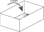
ds n ⋅ J represents the net flux of probability passing through the surface S of the region R. (The symbol n represents a unit vector normal to S.) From (1.3) we can see that if the system is isolated (there is no flow of probability current across any point on the surface of R), then F = 0, so the total probability P is conserved (constant in time). However, if the system is open [there is a flow of probability through the surface of R so that F ≠ 0 (see Fig. 1.1)], then the total probability inside R is not constant. Such a system cannot be in equilibrium.

Fig. 1.1 A system with a net flow of probability into i...

Table of contents

• Cover
• Halftitle
• Title
• Copyright
• Dedication
• Preface
• Preface
• Acknowledgment
• Contents
• Part I. Introduction to PT Symmetry
• Part II. Advanced Topics in PT Symmetry
• Bibliography
• Index