Robust Mixed Model Analysis

Jiming Jiang

• Publisher: WSPC
• Year: 2019
• eBook ISBN: 9789814733854
• Topic: Mathematics
• Subtopic: Probability & Statistics
• Index: Mathematics

Mixed-effects models have found broad applications in various fields. As a result, the interest in learning and using these models is rapidly growing. On the other hand, some of these models, such as the linear mixed models and generalized linear mixed models, are highly parametric, involving distributional assumptions that may not be satisfied in real-life problems. Therefore, it is important, from a practical standpoint, that the methods of inference about these models are robust to violation of model assumptions. Fortunately, there is a full scale of methods currently available that are robust in certain aspects. Learning about these methods is essential for the practice of mixed-effects models.

This research monograph provides a comprehensive account of methods of mixed model analysis that are robust in various aspects, such as to violation of model assumptions, or to outliers. It is suitable as a reference book for a practitioner who uses the mixed-effects models, and a researcher who studies these models. It can also be treated as a graduate text for a course on mixed-effects models and their applications.

Contents:

• Introduction
• Generalized Estimating Equations
• Non-Gaussian Linear Mixed Models
• Robust Tests
• Observed Best Prediction
• Model Selection
• Other Topics

Readership: Graduate students and researchers in statistics and biostatistics. And also those who routinely use mixed-effects models in the fields of genetics, medicine, agriculture, education, and surveys.GEE;Mixed Effects;Model Selection;Non-Gaussian;Prediction;Robust Estimation;Tests0 Key Features:

• It is the first in looking at robust features of existing methods of mixed model analysis
• It covers a wide range of mixed-effects models, including linear mixed models, generalized linear mixed models, semi-parametric and non-parametric mixed models
• It considers different aspects of mixed model analysis, ranging from estimation to tests, and to prediction and model selection

Chapter 1

Introduction

Mixed effects models, or mixed models, have had a wide-ranging impact in modern applied statistics. See, for example, Jiang (2007), McCulloch et al. (2008), Demidenko (2013). These models are characterized by random effects that are involved in a certain way. Depending on how the random effects are involved, a mixed model may be classified as a linear mixed model (LMM), generalized linear mixed model (GLMM), non-linear mixed model (NLMM), semi-parametric mixed model (SPMM), or non-parametric mixed model (NAMMA). Due to their broad applications, there has been a growing interest in learning about these models. On the other hand, some of these models, such as LMM and GLMM, are highly parametric, involving distributional assumptions that may not be satisfied in real-life problems. It is important to make sure that a procedure of statistical analysis is robust against violation of the assumptions, or some “bad cases”. Here the word robustness is formally introduced, for the first time, and we need to make clear what it means. Generally speaking, it means the ability of a procedure to survive some unexpected situations. Life is full of surprises. The unexpected situation could be a violation of an assumption, an outlying observation, or something else. Luckily for the practitioners, there is a rich collection of methods that are currently available and robust, in certain ways. As an introductory example, consider the following.

1.1Illustrative example

A special class of LMM is the mixed ANOVA model [e.g., Jiang (2007)], which can be expressed as

where X is a known matrix of covariates, β is a vector of unknown parameters (the fixed effects), Z₁, . . . , Z_s are known matrices, α₁, . . . , α_s are vectors of random effects, and ϵ is a vector of errors. The standard assumption assumes that

, where

is an unknown variance, 1 ≤ r ≤ s, and I_n denotes the n × n identity matrix, and ϵ ~ N(0, τ²I_N), and that α₁, . . . , α_s, ϵ are independent. Under such assumptions, restricted maximum likelihood (REML) estimators of the fixed effects, β, and variance components,

, 1 ≤ r ≤ s and τ², can be derived. Namely, let A be an N × (N − p) matrix, where p = rank(X), such that

The REML estimator of

is the maximum likelihood (ML) estimator of ψ based on z = A′y, whose distribution does not depend on β. Once the REML estimator of ψ is obtained, say,

, the REML estimator of β is given by

where

. It can be shown (Exercise 1.1) that the REML estimator,

, is a solution to the following REML equations:

where P = V⁻¹ − V⁻¹X(X′V⁻¹X)⁻¹X′V⁻¹ and V is

with

, 1 ≤ r ≤ s and

replaced by

, 1 ≤ r ≤ s and τ², respectively. Here we assume, for simplicity, that X is full rank.

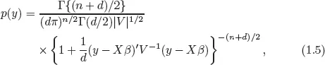
The point to be made is that the REML equations (1.4), which are derived under the normality assumption, can be derived under a completely different distribution. In fact, exactly the same equations will arise if the distribution of y is assumed to be multivariate-t with the probability density function (pdf)

where d is the degree of freedom of the multivariate t-distribution and |V| denotes the determinant of V. Note that the multivariate normal distribution may be viewed as the limiting distribution of the multivariate-t as d → ∞ (Exercise 1.2). An implication is that the Gaussian REML estimator, that is, REML estimator derived under the normality assumption, is still valid even if the normality assumption is violated in that the actual distribution is multivariate-t. The latter is known to have heavier tails than the multivariate normal distribution.

A further question is how far can one go in violating the normality assumption. For example, what if the actual distribution is unknown? We shall address the issue more systematically later.

1.2Outline of approaches to robust mixed model analysis

The simplest way of doing something is not to do anything at all.

Not exactly.

Here by not doing anything it merely means that there is no need to make any changes in the existing procedure to make it robust. Still, one has to justify the robustness of the existing procedure. The justification can be by exact derivation, as in Section 1.1 (also Exercise 1.2), by asymptotic arguments, or by empirical studies, such as Monte-Carlo simulations and real-data applications. This is what we call the first approach.

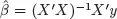
The second approach is to build a procedure of mixed model analysis on weaker assumptions. For example, quasi-likelihood methods avoid full specification of the likelihood function by using estimating functions, or estimating equations. The latter rely only on specification of moments, typically the first two moments. Generally speaking, the more assumptions one makes, the more likely some of these assumptions will be violated. Conversely, a procedure built on weaker assumptions is likely to be more robust than one built on stronger assumptions. Another well-known example is the least squares (LS) method. Under the standard linear regression model, which can be viewed as (1.1) without the term Z₁α₁ + ··· + Z_sα_s, the ML estimator for β is given by

, assuming, again, that X is full rank. However, the same estimator can be derived from a seemingly different principle, the least squares (LS), which does not use the normality assumption at all. In fact, the Gaussian ML estimator remains consistent even if the normality fails [e.g., Jiang (2010), sec. 6.7] and, in this sense, the ML estimation is robust. However, the ML, or LS, estimator has another problem: It is not robust to outliers. This brings up the next approach.

The third approach, which is often considered when dealing with outliers, is to robustify an existing method to make it more robust. Here by robustification it means to modify some part of the current procedure with the intention of robustness. For example, generalized estimating equations (GEE) has been used in the analysis of longitudinal data [e.g., Diggle et al. (2002); see Chapter 2 below]. However, there has been concerns that the GEE may not be robust to outlying observations. One way to robustify the GEE is to modify the definition of the residuals so that it has a bounded range, thus reducing the influence of an outlier.

The next approach is to go semi-parametric, or non-parametric. These models are more flexible, or less restrictive, in some ways so that the chance of model misspecification is (greatly) reduced. For example, instead of assuming a linear mixed-effects function, as in LMM, one may assume that the mean function, conditional on the random effects, is an unknown, smooth function. The latter, of course, includes the linear function as a special case so, when the LMM holds, the non-parametric approach would lose some efficiency. Howe...

Table of contents

• Cover Page
• Title Page
• Copyright Page
• Contents
• Preface
• 1. Introduction
• 2. Generalized Estimating Equations
• 3. Non-Gaussian Linear Mixed Models
• 4. Robust Tests
• 5. Observed Best Prediction
• 6. Model Selection
• 7. Other Topics
• Bibliography
• Index