Chaos in Nature

Christophe Letellier

• Publisher: WSPC
• Year: 2019
• ISBN:
  9789811201219
• Edition: 2
• Topic: Physical Sciences
• Subtopic: Chaotic Behavior in Systems

This book is devoted to the history of chaos theory, from celestial mechanics (three-body problem) to electronics and meteorology. Many illustrative examples of chaotic behaviors exist in various contexts found in nature (chemistry, astrophysics, biomedicine). This book includes the most popular systems from chaos theory (Lorenz, Rössler, van der Pol, Duffing, logistic map, Lozi map, Hénon map etc.) and introduces many other systems, some of them very rarely discussed in textbooks as well as in scientific papers. The contents are formulated with an original approach as compared to other books on chaos theory.

Contents:

• Preface
• Foreword by Otto E Rössler
• Foreword by Robert Gilmore
• Acknowledgments
• From Celestial Mechanics to Chaos:
  • The Laws of Dynamics
  • The Three-Body Problem
  • Simplification of the Three-Body Problem
  • The Success of Celestial Mechanics
  • Birth of the Global Analysis
  • The Stability of the Solar System
• Chaos in Nature: Properties and Examples:
  • Periodic and Chaotic Oscillators
  • From Mathematics to Electronic Circuits
  • From Meteorology to Chaos: The Second Wave
  • The Architecture of Chaotic Attractors
  • Chemical Reactions
  • Population Evolution
  • Chaotic Stars
  • Chaos in Biology and Biomedicine
  • Epilogue
• General Index
• Author Index

Readership: Advanced undergraduates and graduate students in nonlinear dynamics, and non-experts interested in chaos theory. Chaos;Celestial Mechanics;Electronics;Biomedicine;Astrophysics;Lorenz Attarcator;Rossler Attractor0 Key Features:

• Includes historical aspects of key contributions from Rössler, Appleton, Bethe, Lorenz, etc.
• Describes original experimental applications (electrodissolution, Belouso–Zhabotinskii reaction, thermionic diode, Lynx population in the Hudson Bay, sunspots numbers, pulsating stars...)
• All simulations were checked and required information for reproducing them is provided (parameter values, initial conditions, equations)

PART 2

Chaos in Nature: Properties and Examples

Chapter 1

Periodic and Chaotic Oscillators

Chaotic behavior is intimately intertwined with the three-body problem. In celestial mechanics we treat the energy as a conserved quantity because dissipation is negligible since the planets move in a very high vacuum. This is very rarely observed for phenomena that occur on the earth (there is always friction somewhere): systems dissipate energy through heat. The trajectories of such systems are “attracted” to certain regions in their state spaces: these regions correspond to the existence of attractors of the type that we will encounter with the damped pendulum. In this case the attractor is a simple point in the state space that defines a stable state of rest (zero angle, zero angular velocity). There exist much more interesting situations in which the attractor is more complicated (chaotic, for example).

The purpose of this chapter is to describe the fundamental differences between conservative and dissipative dynamical systems. In addition, the manner in which periodic behavior can be understood as superposition of sinusoidal oscillations of different frequencies — Fourier spectrum — will be illustrated with simple examples before we introduce the history of the discoveries that paved the way for the development of the chaos theory.

We will show that sensitivity to initial conditions for dissipative systems is not of the same nature as that encountered for conservative systems, such as the Hénon-Heiles system. In fact, for conservative systems evolving under the same parameter values the motion can be either periodic, quasi-periodic or chaotic, depending on the initial conditions. For a dissipative system the trajectories are organized somewhat differently. Because of energy dissipation there is often a set of initial conditions for which the asymptotic behavior is globally the same. That is, the object in the state space (attractor) towards which typical trajectories evolve is always the same. In other words, for a large number of initial conditions, trajectories converge to the same attractor which they never leave. In fact, as we will see in the case of the damped pendulum, there is a transient regime between the initial conditions and the attractor: this is of little interest for physicists and only the asymptotic behavior will be considered. Under time evolution the attractor for a dissipative system is invariant in the same sense that the torus associated with quasi-periodic motion for a conservative system is invariant: a trajectory in the attractor never leaves it.

1.1Oscillators and Degrees of Freedom

Each mechanical system with n degrees of freedom is associated with a system of n oscillators. The idea of degree of freedom is related to the possible directions of motion. For example, an ideal pendulum oscillating in a plane is a system with one degree of freedom. If the pendulum is now fixed at a point it can move in two directions: this system has two degrees of freedom. In fact, a system consisting of a single body at the end of a rigid rod moving on an axis has a single degree of freedom, if moving on a surface has two degrees of freedom, more complicated pendulum, as double pendulum (two rods and two rotation axes), can move in a volume or a hypervolume, having a large number of degrees of freedom. One can look at other types of systems. For example, two bodies interacting gravitationally (such as the Sun and a planet) has 2 × 2 = 4 degrees of freedom if each body moves in a plane. According to the classical approach, the number of degrees of freedom depends on the number of oscillators needed to describe the system’s motion. For example, an ideal pendulum fixed on a rigid axis is a system with a single degree of freedom, and consequently can be described by a single oscillator.

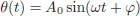
Let us consider a simple case. According to Equation (5.2), the differential equation that describes an ideal pendulum is

The presence of the (nonlinear) sine function complicates the solution of this equation. If we restrict ourselves to small amplitude oscillations, the (nonlinear) term sin θ can be well approximated by the (linear) term θ; then

This equation has for solution

where

is the angular frequency of the pendulum and φ is the phase. The phase permits us to distinguish different trajectories obtained by releasing or pushing on the pendulum from different positions. Thus, small oscillations of the pendulum are correctly described by the term A₀ sin(ωt + φ). The evolution of the pendulum is periodic, that is, it repeats regularly with period

since

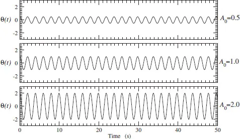
Under this small amplitude approximation, the period of the oscillation does not depend on the amplitude. More precisely, the amplitude of the oscillation at any time t depends only on the amplitude A₀ at t = 0. In Figure 1.1 we show the time evolution of the pendulum for several values of the initial amplitude A₀.

There is a way to determine the period directly from the time evolution of the angle θ as shown, for example, in Figure 1.1: this is from its Fourier spectrum. A Fourier spectrum consists of the set of frequencies that describe the motion: in other words, the time evolution of the angle θ can be decomposed into a sum of oscillating sinusoids with amplitudes A_i, pulsation ω_i¹ and phase φ_i.² There are numerical techniques to estimate parameters A_i, ω_i and φ_i. Fourier spectra provide a representation of amplitude A_i (or of its squared value) versus to the frequency

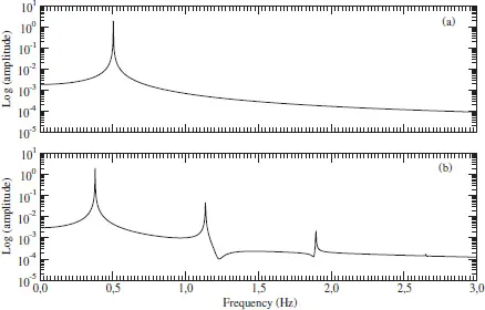
In our pendulum example, when approximation (1.2) is used the motion is exactly sinusoidal at the frequency f₀ = 0.5 Hz: the Fourier spectrum contains just a single frequency (Figure 1.2(a)).

Figure 1.1Evolution of the angle θ that the pendulum makes with the vertical as a function of time for different initial amplitudes A₀ (the pendulum is released at t = 0, thus φ = +π/2). Within the framework of the approximation made for Eq. (1.1) the time period is independent of the initial amplitude.

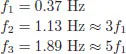
When the approximation of sin θ by θ — replacement of Eq. (1.1) by Eq. (1.2) — cannot be made, the pendulum is described by Eq. (5.3) and the evolution of the angle θ is no longer exactly sinusoidal: two other components with significant amplitudes appear in the Fourier spectrum (Figure 1.2(b)). The time evolution of the pendulum is still periodic but it can be expressed as the sum of three sinusoids:

Figure 1.2Fourier spectra when the time series is (a) a sinusoide and (b) slightly non sinusoidal. Note that in the case where the linear approximation of the sine is no longer used (b), the main frequency (f₁ = 0, 37 Hz) is slightly less than in the case where the approximation is used. (A semi-logarithmic plot is used to better exhibit the various frequencies involved.)

where the angular frequencies ω_i are related to the frequencies f_i by

(here all the phases are zero). The three frequencies are

The amplitudes A_i of the different frequencies decrease very quickly (notice that the plot in Figure 1.2 is semi-logarithmic). This is due to Fourier who showed that every periodic signal could be decomposed into a sum of sinusoids³ in the manner shown in Eq. (1.3).

1.2Damped Pendulum

The pendulum that we have just described is an idealization of a real pendulum. In particular, we have ignored all types of friction, such as friction at the suspension point as well as friction due to motion through the air. Experimentally, moti...