A Practical Approach to XVA

The Evolution of Derivatives Valuation after the Financial Crisis

Osamu Tsuchiya

• Publisher: WSPC
• Year: 2019
• ISBN:
  9789813272750
• Topic: Negocios y empresa
• Subtopic: Ingeniería financiera

The 2008 financial crisis shook the financial derivatives market to its core, revealing a failure to fully price the cost of doing business then. As a response to this, and to cope with regulatory demands for massively increased capital and other measures with funding cost, the pre-2008 concept of Credit Valuation Adjustment (CVA) has evolved into the far more complex hybrid Cross Valuation Adjustment (XVA).

This book presents a clear and concise framework and provides key considerations for the computation of myriad adjustments to the price of financial derivatives, to fully reflect costs. XVA has been of great interest recently due to heavy funding costs (FVA), initial margin (MVA) and capital requirements (KVA) required to sustain a derivatives business since 2008, in addition to the traditional concepts of cost from counterparty default or credit deterioration (CVA), and its mirror image — the cost of one own's default (DVA).

The book takes a practitioner's perspective on the above concepts, and then provides a framework to implement such adjustments in practice. Models are presented too, taking note of what is computationally feasible in light of portfolios typical of investment banks, and the different instruments associated with these portfolios.

Contents:

• Foreword
• Preface
• About the Author
• List of Figures
• List of Tables
• Introduction
• Fundamentals:
  • Underpinnings of Traditional Derivatives Pricing and Implications of Current Environment
• Pricing Adjustments:
  • CVA and its Relation to Traditional Bond Pricing
  • DVA and FVA — Price and Value for Accountants, Regulators and Others
  • Theoretical Framework behind FVA and its Computation
  • Ingredients of the Modern Yield Curve and Overlaps with XVA
  • Margin Valuation Adjustment (MVA)
  • KVA, and Other Adjustments and Costs
• Computing XVA in Practice:
  • Typical Balance Sheet and Trade Relations of Banks and Implication for XVA
  • Framework for Computing XVA
  • Calculation of KVA and MVA
• Managing XVA:
  • CVA Hedging, Default Arrangements and Implications for XVA Modeling
  • Managing XVA in Practice
• Appendices
  • Sample Appendix
  • A Brief Outline of Regulatory Capital Charges for Financial Institutions
• Conclusion
• References
• Index

Readership: Professionals in the financial derivatives industry, as well as graduate students of quantitative finance.XVA;CVA;Valuation Adjustments;Counterparty Credit Risk;CCR;KVA;Regulatory Capital0 Key Features:

• The book presents overview of the fundamental principles of XVA
• The book presents the calculation methodology of XVA as concisely as possible
• The book analyzes the features of XVA in the practice of the derivative trading business

Part I

Fundamentals

Chapter 1

Underpinnings of Traditional Derivatives Pricing and Implications of Current Environment

XVA is valuation adjustments to the traditional (risk-free) derivative valuation. Therefore before discussing XVA, traditional derivatives valuation theory will be briefly explained in this chapter (Tan, 2012).

1.1.Fundamentals of Derivatives Pricing

Derivatives are instruments whose payoffs depend on some other underlyings, hence the name (from “derived”). An example of such a derivative is a forward contract to buy 1 share of Apple stock in 1 year’s time for $800, where the underlying is Apple stock. A slightly more complex example is a call option giving the investor the right to buy 1 share of Apple for $800 in 1 year’s time. Derivatives are also prevalent in other asset classes (interest rates, FX, credit, commodities). It is thus natural to assume that the pricing of derivatives is related to the pricing of the underlyings.

The explosive growth of the derivatives market over the past decades was driven partly by demands of corporates managing risks (primarily interest rates and FX), and also the ability of financial institutions to “synthesize” these instruments, by effectively hedging (i.e. offsetting) some of their risks using simpler underlyings.

Principle: If two portfolios have exactly the same payout under all circumstances at a future date, then they must have the same value.

It follows that to value a derivative of a certain payoff, the approach is to construct a portfolio of simpler instruments which give exactly the same payoff at a future time. The reason for using simpler instruments is because we assume they are more liquidly traded (i.e. a financial institution can obtain a sufficient supply of them for hedging and without paying too high a bid–offer spread). For example, stocks are readily available, as are interest rate swaps (at least for financial institutions).

The two approaches to construct such a portfolio are as follows:

(1)Static replication: Build a portfolio today whose payout at a future date is (at least approximately) equal to the payout of the derivative.

(2)Dynamic replication: Implement a self-financing trading strategy to buy and sell simple instruments, so that the final payout of this portfolio equals the payout of the derivative. Here, the cost incurred in the trading strategy gives the value of the derivative. In general, a model is necessary to inform the trading strategy (i.e. how much of the underlying to hold at a given time subject to market moves).

Static replication is the preferred approach where possible, because it is generally model independent,¹ but unfortunately its applicability is limited to a far smaller set of derivatives.

1.1.1.Assumptions of derivatives pricing

Derivatives pricing, being predicated on hedging, relies heavily on certain assumptions. Some of them are as follows:

(1)Dynamics of underlying.

(2)Existence of liquid market for underlying with enough depth such that hedging a reasonable position is achievable quickly and at minimal cost (bid–offer spread).

(3)Existence of a market to fund one’s position (i.e. borrow if necessary and invest excess cash).

(4)The bank can fund as necessary to buy the derivative and asset at the risk-free rate r(t).

(5)There is no counterparty risk and future payoff will be paid with certainty.

Traditionally, the approach was to assume (2)–(5), and to focus on (1), i.e. getting the correct dynamics of the underlying. We will however see in Section 1.3 how (2) and (3) are becoming questionable as well.

Here, Black and Scholes established the concept of hedging as follows:

Let us suppose we have a derivative that gives us the option to purchase an underlying. Trade continuously in the underlying in order that the hedged portfolio has zero delta (first mathematical derivative with respect to the underlying). This turns out to get rid of the randomness, leading to the hedged portfolio having only a deterministic component, which grows at the risk-free rate.

Let the value of a derivative with underlying price S(t) be V (t, S(t)) and the risk-free short rate be r(t). In the Black–Scholes model, the asset price follows the Geometrical Brownian motion

The Black–Scholes Partial Differential Equation (PDE) is derived by creating a hedging portfolio with value Π(t). The hedging portfolio consists of δ(t) amount of asset, β_V(t) amount of cash to finance the derivative trade and β_S(t) amount of cash to finance the asset, that is

and V (t, S(t)) + Π(t) = 0.

For the portfolio value V (t, S(t)) + Π(t) to be hedged against asset movements, it is necessary for

Because β_V(t) is the cash to fund the derivative, we need

and the amount of cash for funding the asset β_S(t) is given by

In the traditional derivatives pricing theory, the funding rate is assumed to be the risk-free rate r(t), and the following is satisfied:

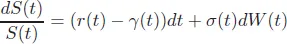
Regarding funding of the money to buy (or sell) underlying stock, there is a dividend yield γ(t) on top of the risk-free funding.²

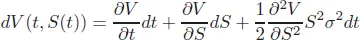
Using Ito’s lemma, by omitting apparent arguments of function, we have

and from the self-financing condition,

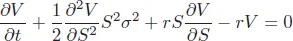
Because d(V (t, S(t)) + Π(t)) = 0, we have the PDE which is called the Black–Scholes equation

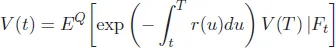
From the Feynman–Kac formula, the solution of the Black–Scholes equation is given by the conditional expectation value as

Here, the expectation value E^Q[ ] is calculated in a probability measure where the asset price process is given by

Implications of Black–Scholes Hedging:

We note that the resultant PDE has a volatility term but not a drift. This immediately leads us to the realization that derivatives pricing is not about predicting the direction in which the underlying will move, since the hedge instruments are supposed to mirror the move.

On the other hand, volatility is relevant because if the underlying is more volatile, hedging has to be conducted more frequently. Roughly, hedging is based on delta, so you buy more when the value of the underlying goes up and sell more when it goes down. Even assuming zero bid–offer spreads, you can only buy when the price has moved from S to S + dS (for an infinitesimal dS), since how would you otherwise know the price is going up? The result of the above is that the hedging strategy costs more when volatility is higher.

But certain limitations of derivatives pricing also stand out given the above details. They are as follows:

(1)Continuity of underlying: Given that we are hedging by getting rid of sensitivity to delta (which only exists if the underlying is continuous), we are clearly assuming a continuous distribution for the underlying. In practice, if the underlying moves sharply, a delta hedge will fail to capture such a move. In practice, a limited set of derivatives have risks that very strongly depend on jumps (e.g. gap risk for CPPI or short-dated options on Credit Default Swaps). The pragmatic approach is often to just add wider margins when in doubt, for cases where dependence is not critical.

(2)Volatility: It should be clear from the above that hedging a long position in optionality is more expensive the higher the volatility. Volatility is not an observable, and hedging cost will depend on realized volatility (from date of trade to expiry of option), whereas an option has to be priced before this cost is known. Thus, whether implied volatility (used to price the option and typically what gets charged to the client) is higher than realized volatility will determine whether selling the derivative is profitable in general.

(3)Funding: What is however less emphasized in academic texts is that there is a funding rate. Typically, this was conveniently thought of as the “risk-free” rate. But financial institutions could never borrow risk-free (even prior to 2008), so this was conveniently thought of as the Libor rate (for AA borrowing) back then. Post 2008 when funding became a far bigger issue, the exact rate to use has become far more important. This will form the heart of our discussion on FVA subsequently.

1.2.Realities of Derivatives Pricing

Even in classical derivatives pricing, the practice of hedging is far less ideal than the theory. As discussed in Section 1.1, it is not generally the case that one needs to have the correct dynamics of an underlying for hedging to work, and in practice it is rare to have the true dynamics of an underlying.

For instance, stock prices will jump (especially downward when bad news affects a company) and volatility will generally get more elevated under such circumstances. To reflect this accurately, it would be necessary to have jumps in the underlying and even stochastic volatility with jumps in the volatility. Such a framework would be totally computationally intractable and is not used in practice. Similarly, short-term interest rates generally jump as central banks adjust their rates in increments of 25 bp. A...

Table of contents

• Cover Page
• Title Page
• Copyright Page
• Dedication
• Foreword
• Preface
• About the Author
• Contents
• List of Figures
• List of Tables
• Introduction
• Part I: Fundamentals
• Part II: Pricing Adjustments
• Part III: Computing XVA in Practice
• Part IV: Managing XVA
• Conclusion
• References
• Index