Applied Linear Regression

Sanford Weisberg

• Publisher: Wiley
• Year: 2013
• Print ISBN: 9781118386088
• eBook ISBN: 9781118594858
• Edition: 4
• Topic: Mathematics
• Subtopic: Applied Mathematics
• Index: Mathematics

Praise for the Third Edition

"...this is an excellent book which could easily be used as a course text..."
—International Statistical Institute

The Fourth Edition of Applied Linear Regression provides a thorough update of the basic theory and methodology of linear regression modeling. Demonstrating the practical applications of linear regression analysis techniques, the Fourth Edition uses interesting, real-world exercises and examples.

Stressing central concepts such as model building, understanding parameters, assessing fit and reliability, and drawing conclusions, the new edition illustrates how to develop estimation, confidence, and testing procedures primarily through the use of least squares regression. While maintaining the accessible appeal of each previous edition,Applied Linear Regression, Fourth Edition features:

• Graphical methods stressed in the initial exploratory phase, analysis phase, and summarization phase of an analysis
• In-depth coverage of parameter estimates in both simple and complex models, transformations, and regression diagnostics
• Newly added material on topics including testing, ANOVA, and variance assumptions
• Updated methodology, such as bootstrapping, cross-validation binomial and Poisson regression, and modern model selection methods

Applied Linear Regression, Fourth Edition is an excellent textbook for upper-undergraduate and graduate-level students, as well as an appropriate reference guide for practitioners and applied statisticians in engineering, business administration, economics, and the social sciences.

CHAPTER 1

Scatterplots and Regression

Regression is the study of dependence. It is used to answer interesting questions about how one or more predictors influence a response. Here are a few typical questions that may be answered using regression:

• Are daughters taller than their mothers?
• Does changing class size affect success of students?
• Can we predict the time of the next eruption of Old Faithful Geyser from the length of the most recent eruption?
• Do changes in diet result in changes in cholesterol level, and if so, do the results depend on other characteristics such as age, sex, and amount of exercise?
• Do countries with higher per person income have lower birth rates than countries with lower income?
• Are highway design characteristics associated with highway accident rates? Can accident rates be lowered by changing design characteristics?
• Is water usage increasing over time?
• Do conservation easements on agricultural property lower land value?

In most of this book, we study the important instance of regression methodology called linear regression. This method is the most commonly used in regression, and virtually all other regression methods build upon an understanding of how linear regression works.

As with most statistical analyses, the goal of regression is to summarize observed data as simply, usefully, and elegantly as possible. A theory may be available in some problems that specifies how the response varies as the values of the predictors change. If theory is lacking, we may need to use the data to help us decide on how to proceed. In either case, an essential first step in regression analysis is to draw appropriate graphs of the data.

We begin in this chapter with the fundamental graphical tools for studying dependence. In regression problems with one predictor and one response, the scatterplot of the response versus the predictor is the starting point for regression analysis. In problems with many predictors, several simple graphs will be required at the beginning of an analysis. A scatterplot matrix is a convenient way to organize looking at many scatterplots at once. We will look at several examples to introduce the main tools for looking at scatterplots and scatterplot matrices and extracting information from them. We will also introduce notation that will be used throughout the book.

1.1 Scatterplots

We begin with a regression problem with one predictor, which we will generically call X, and one response variable, which we will call Y.¹ Data consist of values (x_i, y_i), i = 1, … , n, of (X, Y) observed on each of n units or cases. In any particular problem, both X and Y will have other names that will be displayed in this book using typewriter font, such as temperature or concentration, that are more descriptive of the data that are to be analyzed. The goal of regression is to understand how the values of Y change as X is varied over its range of possible values. A first look at how Y changes as X is varied is available from a scatterplot.

Inheritance of Height

One of the first uses of regression was to study inheritance of traits from generation to generation. During the period 1893–1898, Karl Pearson (1857–1936) organized the collection of n = 1375 heights of mothers in the United Kingdom under the age of 65 and one of their adult daughters over the age of 18. Pearson and Lee (1903) published the data, and we shall use these data to examine inheritance. The data are given in the data file Heights.²

Our interest is in inheritance from the mother to the daughter, so we view the mother's height, called mheight, as the predictor variable and the daughter's height, dheight, as the response variable. Do taller mothers tend to have taller daughters? Do shorter mothers tend to have shorter daughters?

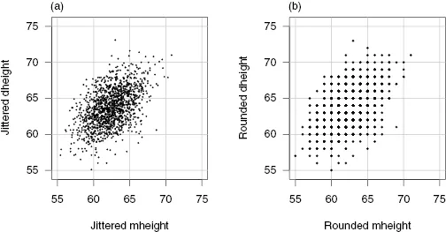
A scatterplot of dheight versus mheight helps us answer these questions. The scatterplot is a graph of each of the n points with the response dheight on the vertical axis and predictor mheight on the horizontal axis. This plot is shown in Figure 1.1a. For regression problems with one predictor X and a response Y, we call the scatterplot of Y versus X a summary graph.

Figure 1.1 Scatterplot of mothers' and daughters' heights in the Pearson and Lee data. The original data have been jittered to avoid overplotting in (a). Plot (b) shows the original data, so each point in the plot refers to one or more mother–daughter pairs.

Here are some important characteristics of this scatterplot:

1. The range of heights appears to be about the same for mothers and for daughters. Because of this, we draw the plot so that the lengths of the horizontal and vertical axes are the same, and the scales are the same. If all mothers and daughters pairs had exactly the same height, then all the points would fall exactly on a 45°-line. Some computer programs for drawing a scatterplot are not smart enough to figure out that the lengths of the axes should be the same, so you might need to resize the plot or to draw it several times.

2. The original data that went into this scatterplot were rounded so each of the heights was given to the nearest inch. The original data are plotted in Figure 1.1b. This plot exhibits substantial overplotting with many points at exactly the same location. This is undesirable because one point on the plot can correspond to many cases. The easiest solution is to use jittering, in which a small uniform random number is added to each value. In Figure 1.1a, we used a uniform random number on the range from −0.5 to +0.5, so the jittered values would round to the numbers given in the original source.

3. One important function of the scatterplot is to decide if we might reasonably assume that the response on the vertical axis is independent of the predictor on the horizontal axis. This is clearly not the case here since as we move across Figure 1.1a from left to right, the scatter of points is different for each value of the predictor. What we mean by this is shown in Figure 1.2, in which we show only points corresponding to mother–daughter pairs with mheight rounding to either 58, 64, or 68 inches. We see that within each of these three strips or slices, the number of points is different, and the mean of dheight is increasing from left to right. The vertical variability in dheight seems to be more or less the same for each of the fixed values of mheight.

4. In Figure 1.1a the scatter of points appears to be more or less elliptically shaped, with the major axis of the ellipse tilted upward, and with more points near the center of the ellipse rather than on the edges. We will see in Section 1.4 that summary graphs that look like this one suggest the use of the simple linear regression model that will be discussed in Chapter 2.

5. Scatterplots are also important for finding separated points. Horizontal separation would occur for a value on the horizontal axis mheight that is either unusually small or unusually large relative to the other values of mheight. Vertical separation would occur for a daughter with dheight either relatively large or small compared with the other daughters with about the same value for mheight.

These two types of separated points have different names and roles in a regression problem. Extreme values on the left and right of the horizontal axis are points that are likely to be important in fitting regression models and are called leverage points. The separated points on the vertical axis, here unusually t...

Table of contents

• Cover
• Wiley Series in Probability and Statistics
• Title page
• Copyright page
• Dedication
• Preface to the Fourth Edition
• CHAPTER 1: Scatterplots and Regression
• CHAPTER 2: Simple Linear Regression
• CHAPTER 3: Multiple Regression
• CHAPTER 4: Interpretation of Main Effects
• CHAPTER 5: Complex Regressors
• CHAPTER 6: Testing and Analysis of Variance
• CHAPTER 7: Variances
• CHAPTER 8: Transformations
• CHAPTER 9: Regression Diagnostics
• CHAPTER 10: Variable Selection
• CHAPTER 11: Nonlinear Regression
• CHAPTER 12: Binomial and Poisson Regression
• Appendix
• References
• Author Index
• Subject Index