Nonlinear Regression Modeling for Engineering Applications

Modeling, Model Validation, and Enabling Design of Experiments

R. Russell Rhinehart

• Publisher: Wiley-ASME Press Series
• Year: 2016
• Print ISBN: 9781118597965
• eBook ISBN: 9781118597958
• Edition: 1
• Topic: Mathematics
• Subtopic: Mathematical Analysis
• Index: Mathematics

Since mathematical models express our understanding of how nature behaves, we use them to validate our understanding of the fundamentals about systems (which could be processes, equipment, procedures, devices, or products). Also, when validated, the model is useful for engineering applications related to diagnosis, design, and optimization.

First, we postulate a mechanism, then derive a model grounded in that mechanistic understanding. If the model does not fit the data, our understanding of the mechanism was wrong or incomplete. Patterns in the residuals can guide model improvement. Alternately, when the model fits the data, our understanding is sufficient and confidently functional for engineering applications.

This book details methods of nonlinear regression, computational algorithms,model validation, interpretation of residuals, and useful experimental design. The focus is on practical applications, with relevant methods supported by fundamental analysis.

This book will assist either the academic or industrial practitioner to properly classify the system, choose between the various available modeling options and regression objectives, design experiments to obtain data capturing critical system behaviors, fit the model parameters based on that data, and statistically characterize the resulting model. The author has used the material in the undergraduate unit operations lab course and in advanced control applications.

Part I

Introduction

Chapter 1
Introductory Concepts

1.1 Illustrative Example – Traditional Linear Least-Squares Regression

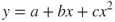
Consider this objective: find the best quadratic model, as described by the following equation:

1.1

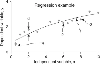
which matches the data in Figure 1.1.

Figure 1.1 Illustration of regression concepts

Here, “x” represents the independent variable and “y” the dependent variable. Often, x and y are respectively termed cause and effect, input and output, influence and response, property and condition, and y is termed a function of x. Equation 1.1 is a human's mathematical description of how y responds to x and it is likely that the relation will not exactly match how nature actually works. In regression, in fitting a model to data, the values of the model coefficients (a, b, and c) will be adjusted to create the best model.

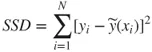
Conventionally, the best model is the one that minimizes the sum of squared distances from data point to model curve, where distance is that for the dependent variable (parallel to the vertical y axis). One data-to-model deviation is indicated as “d” on Figure 1.1. The sum of squared deviations (SSD) is defined as

1.2

where N indicates the number of data points on Figure 1.1 and “i” the number of a particular data point within the set of N. The number associated with a data point does not necessarily correspond with either x or y values. More likely the data point number corresponds to the chronological order of experimental trials that implemented the x value and measured the y response, as the sequential trial number is indicated on Figure 1.1. The data set might appear as illustrated in Table 1.1.

Table 1.1 Illustration of data for Figure 1.1

Trial number	X, Input variable value	Y, Response variable value
1	7.5	2.7
2	6	2.3
3	8	2.6
4	0.5	0.7
.	.	.
.	.	.
.	.	.

Continuing the explanation of Equation 1.2, y_i represents the ith measured y value, the data value, from Table 1.1, and

indicates the model-calculated y value from Equation 1.1 using the ith x value from Table 1.1. The tilde accents on the symbols

and

are both explicit indications that

represents the modeled y value. Redundancy in symbols is often not used, and here the

term will be represented by either

or

.

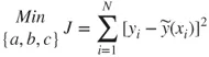
The objective, find values for coefficients a, b, and c that minimize the SSD, defines an optimization procedure. Conventionally, the optimization application is stated by:

1.3

In the jargon of optimization, Equation 1.3 reads, “The objective is to Min(imize) the Objective Function J (equal to the SSD) by adjustment of values of the decision variables (DVs) a, b, and c.” This fully describes the regression “problem.” DVs are what you adjust to minimize the objective function (OF) value. The DVs are the model coefficients that are adjusted to make the model best fit the data.

As a model of the y response to x, Equation 1.1 is nonlinear. Nonlinear means not linear, but does not indicate what the nonlinearity is (quadratic, cubic, reciprocal, exponential, etc.). If the cx² term was not in Equation 1.2 then the model would describe a linear y–x relation. However, in regression we adjust coefficient values, not the x or y values, and in Equation 1.1 each coefficient appears linearly (holding all else constant, the value of y is a linear response to the value of either a or b or c). The exponent for each coefficient is +1 and none of the coefficients are imbedded within a functionality that would make it have a nonlinear impact on y. A formal definition of linearity is given later. Linearity simplifies determination of the optimum values for coefficien...

Table of contents

• Cover
• Wiley-ASME Press Series List
• Title Page
• Copyright
• Table of Contents
• Series Preface
• Preface
• Acknowledgments
• Nomenclature
• Symbols
• Part I: Introduction
• Part II: Preparation for Underlying Skills
• Part III: Regression, Validation, Design
• Part IV: Case Studies and Data
• Appendix A: VBA Primer: Brief on VBA Programming – Excel in Office 2013
• Appendix B: Leapfrogging Optimizer Code for Steady-State Models
• Appendix C: Bootstrapping with Static Model
• References and Further Reading
• Index
• End User License Agreement