Discrete Element Method to Model 3D Continuous Materials

Mohamed Jebahi, Damien Andre, Inigo Terreros, Ivan Iordanoff

• Publisher: Wiley-ISTE
• Year: 2015
• Print ISBN: 9781848217706
• eBook ISBN: 9781119102755
• Edition: 1
• Topic: Technology & Engineering
• Subtopic: Materials Science
• Index: Technology & Engineering

Complex behavior models (plasticity, cracks, visco elascticity) face some theoretical difficulties for the determination of the behavior law at the continuous scale. When homogenization fails to give the right behavior law, a solution is to simulate the material at a meso scale in order to simulate directly a set of discrete properties that are responsible of the macroscopic behavior.  The discrete element model has been developed for granular material. The proposed set shows how this method is capable to solve the problem of complex behavior that are linked to discrete meso scale effects.

1

State of the Art: Discrete Element Modeling

1.1. Introduction

As mentioned in the previous chapter, in conjunction with the accelerating progress in computer science and software technology, the final decades of the 20th Century have seen an explosion of powerful numerical methods which can be classified into discrete methods (DMs) and continuum methods (CMs). These methods have been used over the years to simulate a wide variety of mechanical problems at different scales. Typically, four scales can be distinguished in the context of numerical simulation:

– the nanoscopic (or atomic) scale (∼ 10⁻⁹ m), where phenomena related to the behavior of electrons become significant. At this scale, the interaction between particles (electrons, atoms, etc.) is directly dictated by their quantum mechanical (QM) state;

– the microscopic scale (∼ 10⁻⁶ m), where phenomena related to the behavior of atoms are considered. The interaction between atoms is governed by empirical interatomic potentials, which are generally derived from

QM computations. Classic Newtonian mechanics is used to compute the displacements and rotations of atoms;

– the mesoscopic scale (∼ 10⁻⁴m), where phenomena related to lattice defects are considered. At this scale, the atomic degrees of freedom are not explicitly treated, and only larger scale entities (clusters of atoms, clusters of molecules, etc.) are considered. The interaction between particles is also described by classic Newtonian mechanics;

– the macroscopic scale (∼ 10⁻²m), where macroscopic phenomena which can be described by continuum mechanics are considered. At this scale, the studied physical systems are regarded as continua, whose associated behavior is described by constitutive laws.

Typically, the DMs cover the first three scales. At these scales, the length scale of interest is at the same order of magnitude as the discontinuity spacing, which makes inappropriate the application of traditional CMs. Otherwise, additional handling is required to correctly reproduce phenomena associated with discontinuities like strain localization at crack initiation. At the macroscopic scale, most of the interesting materials can be treated as continua even though they consist of discrete grains at smaller scales. CMs can therefore be used without remorse at this scale. However, it is often rewarding to model such materials as discontinuous by DMs because new knowledge can be gained about their macroscopic behavior when their microscopic mechanisms are understood. The need to model these materials as discontinuous is even more rooted when they are characterized by complex nonlinear mechanical behaviors that cannot easily be described by traditional continuum theories, e.g. anomalous behavior of silica glass [JEB 13b]. This reflects the tremendous diversity of problems to which discrete element modeling can be applied and the ever-increasing availability of DMs. Section 1.2 gives a bird’s-eye view of these methods, in order to position the one that is used in this book; the reader can refer to [DON 09, JIN 07, JEB 14] for more detail. The common feature of these methods is that the studied material is modeled by a set of discrete elements, which can be of different shape and size. These elements interact with each other by contact laws and/or cohesive bonds whose type is directly dictated by the physics of the material being modeled. Knowing forces and torques applied on the discrete elements, displacements and rotations can be computed using the Newton’s second law. For practical purposes, it would be often beneficial to express these results in terms of homogeneous macroscopic variables (e.g. strains and stresses). This allows us, for example, to compare the numerical results with experimental ones. Several techniques have been developed to assess macroscopic quantities from the discrete variables (e.g. force, displacement, etc.). The most commonly used techniques are detailed in section 1.4.

1.2. Classification of discrete methods

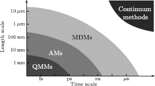
According to the analysis scale, the DMs most commonly used in numerical simulation can be classified into three classes: quantum mechanical (or ab initio) methods (QMMs), atomistic methods (AMs) and mesoscopic DMs (MDMs) (Figure 1.1).

Figure 1.1. Characteristic length scales and time scales for numerical methods

1.2.1. Quantum mechanical methods

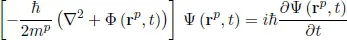
The QMMs are used for material simulation at the atomic scale (∼ 10⁻⁹ m), in which the electrons are the players (Figure 1.1). The molecules are treated as collections of nuclei and electrons whose interaction is directly dictated by their QM state, without any reference to ^“chemical bonds^”. These methods all ultimately stem from the Schrödinger equation first brought to light in 1925. The fully time-dependent form of this equation for a single particle p (e.g. electron) is expressed as:

[1.1]

where m^p and r^p are, respectively, the mass and position vector of the particle of interest, t designates the time, Φ is an external field (e.g. elecrostatic potential), ∇² is the Laplacian, ¯h is Plank’s constant divided by 2π, i is the square root of −1 and Ψ is the wave function which characterizes the particle motion. In fact, the wave function Ψ can properly be obtained for all the particles within a system, which, for crystalline materials, is actually reduced to the primitive unit cell because of translational symmetry. However, equation [1.1] needs this function to be expressed for individual particles. To get around this, the technique most commonly used is to write the overall wave function as a product of single-particle wave functions (the Slater determinant) and then to recast the underlying Schrödinger equation in terms of these functions. Solving this equation gives the particle motions, which in turn give the molecular structure and energy among other observables, as well as information about bonding. The challenge in developing QMMs is that such an equation can be solved exactly only for few problems, e.g. one-electron system (the hydrogen atom), and approximations need to be made. The approximation commonly used is the so-called ^“Hartree–Fock^” which consists of replacing the ^“correct^” description of particle (electron) motions by a picture in which the particles behave essentially as independent bodies. Several other approximations can be found in the literature. These approximations constitute the main difference between QMMs. Examples of these methods are quantum Monte Carlo (QMC) [FOU 01] and quantum chemistry (QC) [SZA 89]. These methods allow us to treat electrons explicitly and accurately, which makes them very accurate but computationally too demanding to handle more than a few tens of electrons. Other QMMs are density-functional theory (DFT) and local density approximation (LDA) [HOH 64, PAY 92]. In these approaches, the primary Schrödinger equation is expressed in terms of particle density rather than the wave functions. Although they are less accurate than QMC or QC, these methods can be readily applied to systems containing several hundred atoms for static properties. Dynamic simulations with DFT and LDA are usually limited to timescales of a few picoseconds.

Overall, the QM methods are generally very accurate since they hold out the possibility of performing simulations without need for prior tuning. However, they are extremely expensive and can only be applied on very small domains a few nanometers in size. Indeed, they deal with electrons in a system and, even if some of the electrons are ignored (as in the semi-empirical approaches), a large number of particles must still be considered.

1.2.2. Atomistic methods

The AMs are used for material simulation at the microscopic scale (∼ 10⁻⁶ m), where atoms are the players (Figure 1.1). These methods ignore the electronic motions and compute the energy of a system as a function of the atomic positions only. This way to compute energy derives its legitimacy from the Born–Oppenheimer approximation, which postulates that the electrons adjust to the new atomic positions much faster than the atomic nuclei. The interaction laws between particles (atoms) can be described by empirical interatomic potentials that encapsulate the effects of bonding (mediated by electrons) between them. These potentials may depend on the distance between particles, angles between bonds, angles between pla...

Table of contents

• Cover
• Contents
• Title Page
• Copyright
• List of Figures
• List of Tables
• Preface
• Introduction
• 1 State of the Art: Discrete Element Modeling
• 2 Discrete Element Modeling of Mechanical Behavior of Continuous Materials
• 3 Discrete Element Modeling of Thermal Behavior of Continuous Materials
• 4 Discrete Element Modeling of Brittle Fracture
• Conclusion
• Bibliography
• Index