![]()
Chapter 1
Recap on Digital Signal Processing
Signal processing consists of handling data in order to extract information considered relevant, or to modify them so as to give them useful properties: extracting, for example, information on a plane’s speed or distance from a RADAR signal, making an old and decayed sound recording clearer, synthesizing a sentence on an answering machine, transmitting information through a communication channel, etc.
The processing is called digital if it deals with a discrete sequence of values {x1, x2, ...}. There are two types of scenario: either the observation is already a sequence of numbers, as is the case for example for economic data, either the observed phenomenon is “continuous-time”, and the signal’s value x(t) must then be measured at regular intervals.
This second scenario has tremendous practical applications. This is why an entire section of this chapter is devoted to the operation called sampling.
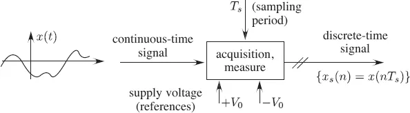
The acquisition chain is described in Figure 1.1.
Figure 1.1 – Digital signal acquisition
The essential part of the acquisition device is usually the analog-to-digital converter, or ADC, which samples the value of the input voltage at regular intervals – every Ts seconds – and provides a coded representation at the output.
To be absolutely correct, this coded value is not exactly equal to the value of x(nTs). However, in the course of this chapter, we will assume that xs(n) = x(nTs). The sequence of these numerical values will be referred to as the digital signal, or more plainly as the signal.
Ts is called the sampling period and Fs = 1/Ts the sampling frequency. The gap between the actual value and the coded value is called quantization noise.
Obviously, the sampling frequency must be high enough “in order not to lose too much information” – a concept we will discuss later on – from the original signal, and there is a connection between this frequency and the sampled signal’s “frequential content”. Anybody who conducts experiments knows this “graph plotting principle”: when the signal’s value changes quickly (presence of “high frequencies”), “many” points have to be plotted (it would actually be preferable to use the phrase “high point density”), whereas when the signal’s value changes slowly (presence of low frequencies), fewer points need to be plotted.
To sum up, the signal sampling must be done in such a way that the numerical sequence {xs(n)} alone is enough to reconstruct the continuous-time signal. The sampling theorem specifies the conditions that need to be met for perfect reconstruction to be possible.
1.1 The sampling theorem
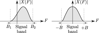
Let x(t) be a continuous signal, with X(F) its Fourier transform, which will also be called the spectrum. The sample sequence measured at the frequency Fs = 1/Ts is denoted by xs(n) = x(nTs).
Definition 1.1 When X(
F)
0 for F (
B1,
B2)
and X(
F) = 0
everywhere else, x(
t)
is said to be (
B1,
B2)
band-limited. If x(
t)
is real, its Fourier transform has a property called Hermitian symmetry,
meaning that X(
F) =
X*(
–F),
and the frequency band’s expression is (–
B, +
B).
A common misuse of language consists of referring to the signal as a B-band signal. Perfect reconstruction
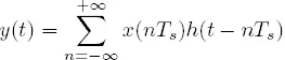
Our goal is to reconstruct x(t), at every time t, using the sampling sequence xs(n) = x(nTs), while imposing a “reconstruction scheme” defined by the expression (1.1):
Figure 1.2 – Spectra of band-limited signals
where h(t) is called a reconstruction function. Notice that (1.1) is linear with respect to x(nTs). In order to reach this objective, two questions have to be answered:
1. is there a class of signals x(t) large enough for y(t) to be identi...