Hands-On Machine Learning with R

Brad Boehmke, Brandon M. Greenwell

• Editorial: Chapman and Hall/CRC
• Año: 2019
• ISBN:
  9781000730432
• Edición: 1
• Categoría: Economics
• Categoría: Statistics for Business & Economics

Hands-on Machine Learning with R provides a practical and applied approach to learning and developing intuition into today's most popular machine learning methods. This book serves as a practitioner's guide to the machine learning process and is meant to help the reader learn to apply the machine learning stack within R, which includes using various R packages such as glmnet, h2o, ranger, xgboost, keras, and others to effectively model and gain insight from their data. The book favors a hands-on approach, providing an intuitive understanding of machine learning concepts through concrete examples and just a little bit of theory.

Throughout this book, the reader will be exposed to the entire machine learning process including feature engineering, resampling, hyperparameter tuning, model evaluation, and interpretation. The reader will be exposed to powerful algorithms such as regularized regression, random forests, gradient boosting machines, deep learning, generalized low rank models, and more! By favoring a hands-on approach and using real word data, the reader will gain an intuitive understanding of the architectures and engines that drive these algorithms and packages, understand when and how to tune the various hyperparameters, and be able to interpret model results. By the end of this book, the reader should have a firm grasp of R's machine learning stack and be able to implement a systematic approach for producing high quality modeling results.

Features:

· Offers a practical and applied introduction to the most popular machine learning methods.

· Topics covered include feature engineering, resampling, deep learning and more.

· Uses a hands-on approach and real world data.

Part II

Supervised Learning

4

Linear Regression

Linear regression, a staple of classical statistical modeling, is one of the simplest algorithms for doing supervised learning. Though it may seem somewhat dull compared to some of the more modern statistical learning approaches described in later chapters, linear regression is still a useful and widely applied statistical learning method. Moreover, it serves as a good starting point for more advanced approaches; as we will see in later chapters, many of the more sophisticated statistical learning approaches can be seen as generalizations to or extensions of ordinary linear regression. Consequently, it is important to have a good understanding of linear regression before studying more complex learning methods. This chapter introduces linear regression with an emphasis on prediction, rather than inference. An excellent and comprehensive overview of linear regression is provided in Kutner et al. (2005). See Faraway (2016b) for a discussion of linear regression in R (the book’s website also provides Python scripts).

4.1 Prerequisites

This chapter leverages the following packages:

# Helper packages

library(dplyr) # for data manipulation

library(ggplot2) # for awesome graphics

# Modeling packages

library(caret) # for cross-validation, etc.

# Model interpretability packages

library(vip) # variable importance

We’ll also continue working with the ames_train data set created in Section 2.7.

4.2 Simple linear regression

Pearson’s correlation coefficient is often used to quantify the strength of the linear association between two continuous variables. In this section, we seek to fully characterize that linear relationship. Simple linear regression (SLR) assumes that the statistical relationship between two continuous variables (say X and Y) is (at least approximately) linear:

$Y_i={\beta }_0+{\beta }_1{X}_i+{ϵ}_i,\text{for}i=1,2,\mathrm{\dots },n,$

(4.1)

where Y_i represents the i-th response value, X_i represents the i-th feature value, β₀ and β₁ are fixed, but unknown constants (commonly referred to as coefficients or parameters) that represent the intercept and slope of the regression line, respectively, and ϵ_i represents noise or random error. In this chapter, we’ll assume that the errors are normally distributed with mean zero and constant variance σ², denoted $\stackrel{iid}{\sim }$ (0, σ²). Since the random errors are centered around zero (i.e., E (ϵ) = 0), linear regression is really a problem of estimating a conditional mean:

$E(Y_i|X_i)={\beta }_0+{\beta }_1{X}_i.$

(4.2)

For brevity, we often drop the conditional piece and write E (Y|X) = E (Y). Consequently, the interpretation of the coefficients is in terms of the average, or mean response. For example, the intercept β₀ represents the average response value when X = 0 (it is often not meaningful or of interest and is sometimes referred to as a bias term). The slope β₁ represents the increase in the average response per one-unit increase in X (i.e., it is a rate of change).

4.2.1 Estimation

Ideally, we want estimates of β₀ and β₁ that give us the “best fitting” line. But what is meant by “best fitting”? The most common approach is to use the method of least squares (LS) estimation; this form of linear regression is often referred to as ordinary least squares (OLS) regression. There are multiple ways to measure “best fitting”, but the LS criterion finds the “best fitting” line by minimizing the residual sum of squares (RSS):

$RSS({\beta }_0,{\beta }_1)={\displaystyle \sum _{i=1}^n{[Y_i-({\beta }_0+{\beta }_1{X}_i)]}^2={\displaystyle \sum _{i=1}^n{(Y_i-{\beta }_0-{\beta }_1{X}_i)}^2}}.$

(4.3)

The LS estimates of β₀ and β₁ are denoted as β̂₀ and β̂₁, respectively. Once obtained, we can generate predicted values, say at X = X_new, using the estimated regression equation:

${\widehat{Y}}_{new}={\widehat{\beta }}_0+{\widehat{\beta }}_1{X}_{new},$

(4.4)

where ${\widehat{Y}}_{new}=E(Y_{new}|\stackrel{⌢}{X}=X_{new})$ is the estimated mean response at X = X_new.

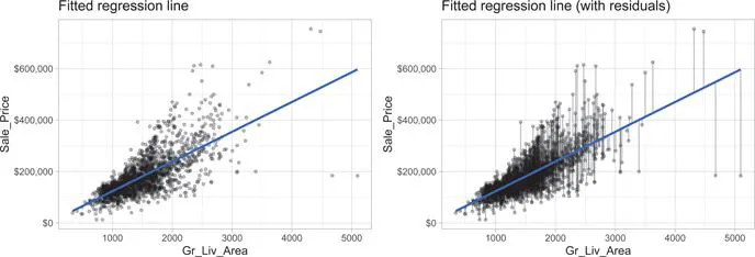
With the Ames housing data, suppose we wanted to model a linear relationship between the total above ground living space of a home (Gr_Liv_Area) and sale price (Sale_Price). To perform an OLS regression model in R we can use the lm() function:

model1 <- lm(Sale_Price ~ Gr_Liv_Area, data = ames_train)

The fitted model (model1) is displayed in the left plot in Figure 4.1 where the points represent the values of Sale_Price in the training data. In the right plot of Figure 4.1, the vertical lines represent the individual errors, called residuals, associated with each observation. The OLS criterion in Equation (4.3) identifies the “best fitting” line that minimizes the sum of squares of these residuals.

FIGURE 4.1: The least squares fit from regressing sale price on living space for the the Ames housing data. Left: Fitted regressi...