2.1 The diffusion tensor and the diffusion ellipsoid
MRI is an imaging technique that detects proton signals from water molecules. Images thus reflect water density and properties as a function of position in space. In addition, MRI can be used to measure the local chemical and physical properties of water. Two such properties are molecular diffusion and flow. MRI can assess both, but the measurement methods are different for each, and they should not be confused.
The diffusion process is a reflection of thermal Brownian motion. This process can be understood in a simple manner by comparing it to the evolution in the shape of a stain after ink is dropped on a piece of paper. Usually, the drop turns into a circle (Gaussian distribution) that grows over time. The faster the diffusion is, the larger the diameter of the circle, and the extent of the diffusion can be estimated from this. Because the extent of the stain is equivalent in all directions, the diffusion is called isotropic. However, if the paper consists of a special fabric that is woven with dense vertical fibers and sparse horizontal fibers, the stain will have an oval shape elongated along the vertical axis. This is called anisotropic diffusion. A similar process happens in the brain where water tends to diffuse preferentially along axonal fibers. If ink were injected inside the brain white matter, the shape of its distribution would be elongated along the axonal tracts. Inside the gray matter, the diffusion process is more random because of the lack of aligned fiber structures, and the shape of the ink would be more spherical.
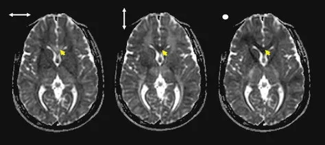
One of the unique aspects of diffusion measurements by MRI is that the extent of water diffusion can be measured along one predetermined axis and this axis can be set arbitrarily. Diffusion measurements can be combined with imaging, from which the effective diffusion constant at each pixel can be measured (called an apparent diffusion constant map). Examples of such diffusion constant maps are shown in Fig. 1. From these images, it can be clearly seen that water diffusion inside the brain is anisotropic: the extent of the measured diffusion constants depends on the measurement orientation, especially in the white matter.
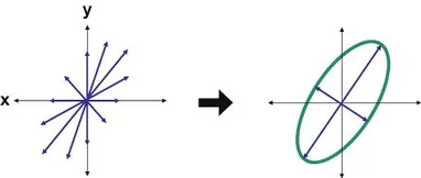
The extent of anisotropy of the water diffusion can be delineated in more detail by measuring the diffusion constant along multiple axes. Due to the complexity of the underlying cytoarchitecture (in addition to noise), the measurements may yield a very complex pattern of anisotropy. However, if there is a homogeneous cytoarchitecture within a pixel (typically 2 × 2 × 2 mm3 or larger, the magnitude of diffusion (or the shape of ink in our analogy) can be described by a simple symmetric 3D ellipsoid (Fig. 2).
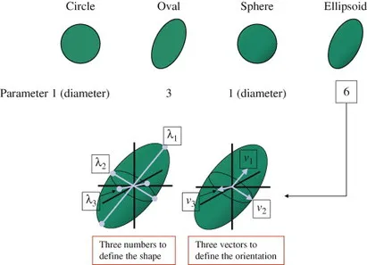
Diffusion tensor imaging is a technique in which diffusion is measured in a series of different spatial directions, from which the shape and orientation of the diffusion ellipsoid is determined at each image pixel by fitting the measurement results obtained in the reference frame of the scanner to the ellipsoid that describes the average local cytoarchitecture. During this measurement and fitting process, we use a 3 × 3 tensor, from which the name, diffusion tensor imaging, is derived. The fitting process for determining the ellipsoid is a mathematical process called diagonalization of the tensor. The 3 × 3 diffusion tensor has nine elements, but there are only six independent numbers because the diffusion tensor is a symmetric tensor, which makes sense, given the fact that the tensor uniquely determines the diffusion ellipsoid. Six parameters are needed to completely describe the magnitude and orientation of the 3D ellipsoid (Fig. 3), and the determination of these six parameters is the target of DTI. Thus, determination of the tensor elements requires measurement of diffusion constants along at least six spatial directions.
2.2 Two-dimensional visualization of DTI results
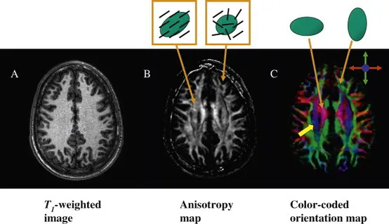
Once the six tensor parameters are determined at each pixel, the information is usually reduced to produce different types of images that can be appreciated visually. It is almost impossible to visualize all six parameters in an intuitive way in a single image, and there are two types of presentations that are generally used. One is the anisotropy map and the other is the orientation map or color map. The anisotropy map provides information about the extent of elongation (anisotropy) of the diffusion ellipsoid (Fig. 4B). In this kind of map, the white matter appears brighter (more anisotropic) than the gray matter, showing brain areas with coherent fiber structures. It is believed that such factors as axonal density, myelination, and homogeneity in the axonal orientation affect the degree of diffusion anisotropy. In the color map, the angle of the longest axis of the ellipsoid (v1 in Fig. 3) is visualized using three principal colors (red (R), green (G), and blue (B)), under the assumption that this is indicative of the dominant fiber orientation (Fig. 4C). The signal intensity is weighted by the diffusion anisotropy. In this kind of map, any arbitrary angle can be represented by a mixture of RGB colors. For example, in Fig. 4, fibers running 45° between the right–left (red) and anterior–posterior (green) axes would be labeled by a yellow (red + green) color.
By comparing these three images, it is clear that the color-coded orientation map carries, by far, the greatest amount of information regarding white matter anatomy. In the conventional T1-weighted MR image on the left, the white matter presents as a homo-geneous field, whereas many internal structures are visible in the color map. For example, the blue-colored fiber indicated by a yellow arrow in Fig. 4C is the corona radiata, which could not be identified in the T1-weighted image. Thus, DTI can be used to parcellate the white matter into substructures.
There is one important limitation of DTI that is essential to understand when reading color maps. This is due to the DTI assumption that there is a homogeneous fiber structure within a pixel. Because of the relatively large size of the pixels in DTI data (2–3 mm), a pi...