MRI Atlas of Human White Matter

Kenichi Oishi, Andreia V. Faria, Peter C M van Zijl, Susumu Mori

• Publisher: Academic Press
• Year: 2010
• ISBN:
  9780123820822
• Edition: 2
• Topic: Biological Sciences
• Subtopic: Neuroscience
• Index: Biological Sciences

MRI Atlas of Human White Matter presents an atlas to the human brain on the basis of T 1-weighted imaging and diffusion tensor imaging. A general background on magnetic resonance imaging is provided, as well as the basics of diffusion tensor imaging. An overview of the principles and limitations in using this methodology in fiber tracking is included.

This book describes the core white-matter structures, as well as the superficial white matter, the deep gray matter, and the cortex. It also presents a three-dimensional reconstruction and atlas of the brain white-matter tracts. The Montreal Neurological Institute coordinates, which are the most widely used, are adopted in this book as the primary coordinate system. The Talairach coordinate system is used as the secondary coordinate system. Based on magnetic resonance imaging and diffusion tensor imaging, the book offers a full segmentation of 220 white-matter and gray-matter structures with boundaries.

• Visualization of brain white matter anatomy via 3D diffusion tensor imaging (DTI) contrasts and enhances relationship of anatomy to function
• Full segmentation of 170+ brain regions more clearly defines structure boundaries than previous point-and-annotate anatomical labeling, andconnectivity is mapped in a way not provided by traditional atlases

Chapter 1 Introduction

We present a human brain atlas based on co-registered T₁-weighted imaging and diffusion tensor imaging (DTI). The conventional T₁-weighted MRI provides a high-resolution view of gray matter anatomy, while the DTI provides unique contrast to decipher the complicated architecture of the white matter. In order to appreciate the images in this atlas, it is necessary to understand how these contrasts are generated. In this section, we provide some general MRI background, followed by the basics of DTI, and an overview of the principles and limitations of fiber tracking using this methodology.

1 Magnetic resonance imaging (MRI)

Magnetic resonance (MR) images consist of individual picture elements (pixels) with different intensities (brightness). When evaluating MR images, two important parameters need to be considered: spatial resolution and contrast. In modern MRI, the spatial resolution (pixel size) is on the order of 1–3 mm or even smaller, revealing a large amount of detail about brain anatomy. Contrast is created by differences in pixel intensities among different areas of the brain. Conventionally, MR contrast has been mostly based on differences in tissue water relaxation times, such as T₁ and T₂, which can be used to distinguish various brain regions, such as the cortex, the deep gray matter, and the white matter. However, conventional MR has not been successful in providing good contrast within the white matter, which usually looks rather homogeneous, no matter how high the spatial resolution. From an MRI point of view, the white matter generally appears as a fluid-like homogeneous structure, which, of course, is not the case.

The white matter consists of axons that connect different areas of the brain. These axons tend to form “bundles,” together with other axons, and, depending on the destinations, the diameters of these bundles (called white matter tracts) can be as large as a few centimeters. Some of them, such as the corpus callosum and the anterior commissure at the mid-sagittal level, are clearly visible on conventional MRI. However, most of these bundles cannot be individually identified by MRI or even with postmortem brain slices. This is because the majority of these bundles have similar chemical compositions and MR signatures (T₁ and T₂ relaxation times). It is very difficult to appreciate where the specific white matter tracts of interest are and how they are spatially related to one another. Actually, conventional MRI is also unable to provide a high level of contrast for intra-gray matter structures. Differences in cytoarchitecture among different cortical layers or between cortical areas cannot be distinguished. Nevertheless, gyral and sulcal patterns can be used as visual clues for cortical anatomy discrimination. Unfortunately, equivalent visual clues are often not available for the identification of white matter tracts.

2 Diffusion tensor imaging (DTI)

2.1 The diffusion tensor and the diffusion ellipsoid

MRI is an imaging technique that detects proton signals from water molecules. Images thus reflect water density and properties as a function of position in space. In addition, MRI can be used to measure the local chemical and physical properties of water. Two such properties are molecular diffusion and flow. MRI can assess both, but the measurement methods are different for each, and they should not be confused.

The diffusion process is a reflection of thermal Brownian motion. This process can be understood in a simple manner by comparing it to the evolution in the shape of a stain after ink is dropped on a piece of paper. Usually, the drop turns into a circle (Gaussian distribution) that grows over time. The faster the diffusion is, the larger the diameter of the circle, and the extent of the diffusion can be estimated from this. Because the extent of the stain is equivalent in all directions, the diffusion is called isotropic. However, if the paper consists of a special fabric that is woven with dense vertical fibers and sparse horizontal fibers, the stain will have an oval shape elongated along the vertical axis. This is called anisotropic diffusion. A similar process happens in the brain where water tends to diffuse preferentially along axonal fibers. If ink were injected inside the brain white matter, the shape of its distribution would be elongated along the axonal tracts. Inside the gray matter, the diffusion process is more random because of the lack of aligned fiber structures, and the shape of the ink would be more spherical.

One of the unique aspects of diffusion measurements by MRI is that the extent of water diffusion can be measured along one predetermined axis and this axis can be set arbitrarily. Diffusion measurements can be combined with imaging, from which the effective diffusion constant at each pixel can be measured (called an apparent diffusion constant map). Examples of such diffusion constant maps are shown in Fig. 1. From these images, it can be clearly seen that water diffusion inside the brain is anisotropic: the extent of the measured diffusion constants depends on the measurement orientation, especially in the white matter.

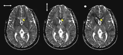
Fig. 1 Diffusion constant maps of the same slice measured along three different orientations (indicated by arrows). For the third image, the orientation is perpendicular to the plane. In these images, brightness represents the extent of diffusion (magnitude of the diffusion constant). Diffusion in white matter is more anisotropic than that in gray matter. For example, the corpus callosum (yellow arrows) has a high diffusion constant when water diffusion is measured along the horizontal axis (first image), but a low diffusion constant when applying diffusion weighting along the vertical axis (second image) or perpendicular to the plane (third image).

The extent of anisotropy of the water diffusion can be delineated in more detail by measuring the diffusion constant along multiple axes. Due to the complexity of the underlying cytoarchitecture (in addition to noise), the measurements may yield a very complex pattern of anisotropy. However, if there is a homogeneous cytoarchitecture within a pixel (typically 2 × 2 × 2 mm³ or larger, the magnitude of diffusion (or the shape of ink in our analogy) can be described by a simple symmetric 3D ellipsoid (Fig. 2).

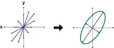
Fig. 2 Using diffusion measurements along multiple axes (left, the length of blue arrows represent the magnitude of diffusion constants), the anisotropic diffusion process can be delineated in detail. In diffusion tensor imaging, the measurement results are fitted to a simple symmetric 3D ellipsoid (or oval in this 2D simplified representation).

Diffusion tensor imaging is a technique in which diffusion is measured in a series of different spatial directions, from which the shape and orientation of the diffusion ellipsoid is determined at each image pixel by fitting the measurement results obtained in the reference frame of the scanner to the ellipsoid that describes the average local cytoarchitecture. During this measurement and fitting process, we use a 3 × 3 tensor, from which the name, diffusion tensor imaging, is derived. The fitting process for determining the ellipsoid is a mathematical process called diagonalization of the tensor. The 3 × 3 diffusion tensor has nine elements, but there are only six independent numbers because the diffusion tensor is a symmetric tensor, which makes sense, given the fact that the tensor uniquely determines the diffusion ellipsoid. Six parameters are needed to completely describe the magnitude and orientation of the 3D ellipsoid (Fig. 3), and the determination of these six parameters is the target of DTI. Thus, determination of the tensor elements requires measurement of diffusion constants along at least six spatial directions.

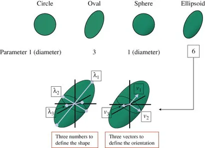
Fig. 3 Parameters required to mathematically describe a circle, oval, sphere, and ellipsoid. The six parameters required for an ellipsoid are three eigenvalues (λ1, λ2, and λ3) that define the shape of the ellipsoid and three eigenvectors (v1, v2, and v3) that define the orientation of the ellipsoid.

2.2 Two-dimensional visualization of DTI results

Once the six tensor parameters are determined at each pixel, the information is usually reduced to produce different types of images that can be appreciated visually. It is almost impossible to visualize all six parameters in an intuitive way in a single image, and there are two types of presentations that are generally used. One is the anisotropy map and the other is the orientation map or color map. The anisotropy map provides information about the extent of elongation (anisotropy) of the diffusion ellipsoid (Fig. 4B). In this kind of map, the white matter appears brighter (more anisotropic) than the gray matter, showing brain areas with coherent fiber structures. It is believed that such factors as axonal density, myelination, and homogeneity in the axonal orientation affect the degree of diffusion anisotropy. In the color map, the angle of the longest axis of the ellipsoid (v1 in Fig. 3) is visualized using three principal colors (red (R), green (G), and blue (B)), under the assumption that this is indicative of the dominant fiber orientation (Fig. 4C). The signal intensity is weighted by the diffusion anisotropy. In this kind of map, any arbitrary angle can be represented by a mixture of RGB colors. For example, in Fig. 4, fibers running 45° between the right–left (red) and anterior–posterior (green) axes would be labeled by a yellow (red + green) color.

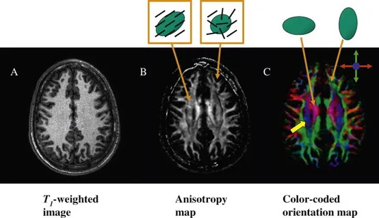
Fig. 4 Examples of (A) conventional MRI (T₁-weighted image), (B) anisotropy map, and (C) color-coded orientation map. For the color-coded images, the intensity (brightness) is proportional to the anisotropy information (same as in anisotropy map, B) and the different colors, red, green, and blue, represent fibers running along the right–left, anterior–posterior, and inferior–superior axes, respectively.

By comparing these three images, it is clear that the color-coded orientation map carries, by far, the greatest amount of information regarding white matter anatomy. In the conventional T₁-weighted MR image on the left, the white matter presents as a homo-geneous field, whereas many internal structures are visible in the color map. For example, the blue-colored fiber indicated by a yellow arrow in Fig. 4C is the corona radiata, which could not be identified in the T₁-weighted image. Thus, DTI can be used to parcellate the white matter into substructures.

There is one important limitation of DTI that is essential to understand when reading color maps. This is due to the DTI assumption that there is a homogeneous fiber structure within a pixel. Because of the relatively large size of the pixels in DTI data (2–3 mm), a pi...