Digital Signal Processing: A Practical Guide for Engineers and Scientists
Steven Smith
This is a test
This is a test
Partager le livre
672 pages
English
ePUB (adapté aux mobiles)
Disponible sur iOS et Android
eBook - ePub
Digital Signal Processing: A Practical Guide for Engineers and Scientists
Steven Smith
Détails du livre
Aperçu du livre
Table des matières
Citations
À propos de ce livre
In addition to its thorough coverage of DSP design and programming techniques, Smith also covers the operation and usage of DSP chips. He uses Analog Devices' popular DSP chip family as design examples.
Covers all major DSP topics
Full of insider information and shortcuts
Basic techniques and algorithms explained without complex numbers
Foire aux questions
Comment puis-je résilier mon abonnement ?
Il vous suffit de vous rendre dans la section compte dans paramètres et de cliquer sur « Résilier l’abonnement ». C’est aussi simple que cela ! Une fois que vous aurez résilié votre abonnement, il restera actif pour le reste de la période pour laquelle vous avez payé. Découvrez-en plus ici.
Puis-je / comment puis-je télécharger des livres ?
Pour le moment, tous nos livres en format ePub adaptés aux mobiles peuvent être téléchargés via l’application. La plupart de nos PDF sont également disponibles en téléchargement et les autres seront téléchargeables très prochainement. Découvrez-en plus ici.
Quelle est la différence entre les formules tarifaires ?
Les deux abonnements vous donnent un accès complet à la bibliothèque et à toutes les fonctionnalités de Perlego. Les seules différences sont les tarifs ainsi que la période d’abonnement : avec l’abonnement annuel, vous économiserez environ 30 % par rapport à 12 mois d’abonnement mensuel.
Qu’est-ce que Perlego ?
Nous sommes un service d’abonnement à des ouvrages universitaires en ligne, où vous pouvez accéder à toute une bibliothèque pour un prix inférieur à celui d’un seul livre par mois. Avec plus d’un million de livres sur plus de 1 000 sujets, nous avons ce qu’il vous faut ! Découvrez-en plus ici.
Prenez-vous en charge la synthèse vocale ?
Recherchez le symbole Écouter sur votre prochain livre pour voir si vous pouvez l’écouter. L’outil Écouter lit le texte à haute voix pour vous, en surlignant le passage qui est en cours de lecture. Vous pouvez le mettre sur pause, l’accélérer ou le ralentir. Découvrez-en plus ici.
Est-ce que Digital Signal Processing: A Practical Guide for Engineers and Scientists est un PDF/ePUB en ligne ?
Oui, vous pouvez accéder à Digital Signal Processing: A Practical Guide for Engineers and Scientists par Steven Smith en format PDF et/ou ePUB ainsi qu’à d’autres livres populaires dans Technology & Engineering et Signals & Signal Processing. Nous disposons de plus d’un million d’ouvrages à découvrir dans notre catalogue.
Most DSP techniques are based on a divide-and-conquer strategy called superposition. The signal being processed is broken into simple components, each component is processed individually, and the results reunited. This approach has the tremendous power of breaking a single complicated problem into many easy ones. Superposition can only be used with linear systems, a term meaning that certain mathematical rules apply. Fortunately, most of the applications encountered in science and engineering fall into this category. This chapter presents the foundation of DSP: what it means for a system to be linear, various ways for breaking signals into simpler components, and how superposition provides a variety of signal processing techniques.
Signals and Systems
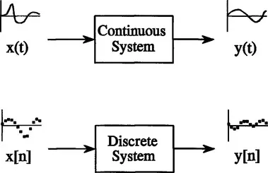
A signal is a description of how one parameter varies with another parameter: for instance, voltage changing over time in an electronic circuit, or brightness varying with distance in an image. A system is any process that produces an output signal in response to an input signal. This is illustrated by the block diagram in Fig. 5-1. Continuous systems input and output continuous signals, such as in analog electronics. Discrete systems input and output discrete signals, such as computer programs that manipulate the values stored in arrays.
FIGURE 5-1 Terminology for signals and systems. A system is any process that generates an output signal in response to an input signal. Continuous signals are usually represented with parentheses, while discrete signals use brackets. All signals use lower-case letters, reserving the upper case for the frequency domain (presented in later chapters). Unless there is a better name available, the input signal is called: x(t) or x[n], while the output is called: y(t) or y[n].
Several rules are used for naming signals. These aren’t always followed in DSP, but they are very common and you should memorize them. The mathematics is difficult enough without a clear notation. First, continuous signals use parentheses, such as: x(t) and y(t), while discrete signals use brackets, as in: x[n] and y[n]. Second, signals use lower-case letters. Uppercase letters are reserved for the frequency domain, discussed in later chapters. Third, the name given to a signal is usually descriptive of the parameters it represents. For example, a voltage depending on time might be called: v(t), or a stock market price measured each day could be: p[d].
Signals and systems are frequently discussed without knowing the exact parameters being represented. This is the same as using x and y in algebra, without assigning a physical meaning to the variables. This brings in a fourth rule for naming signals. If a more descriptive name is not available, the input signal to a discrete system is usually called: x[n], and the output signal: y[n]. For continuous systems, the signals: x(t) and y(t) are used.
There are many reasons for wanting to understand a system. For example, you may want to design a system to remove noise in an electrocardiogram, sharpen an out-of-focus image, or remove echoes in an audio recording. In other cases, the system might have a distortion or interfering effect that you need to characterize or measure. For instance, when you speak into a telephone, you expect the other person to hear something that resembles your voice. Unfortunately, the input signal to a transmission line is seldom identical to the output signal. If you understand how the transmission line (the system) is changing the signal, maybe you can compensate for its effect. In still other cases, the system may represent some physical process that you want to study or analyze. Radar and sonar are good examples of this. These methods operate by comparing the transmitted and reflected signals to find the characteristics of a remote object. In terms of system theory, the problem is to find the system that changes the transmitted signal into the received signal.
At first glance, it may seem an overwhelming task to understand all of the possible systems in the world. Fortunately, most useful systems fall into a category called linear systems. This fact is extremely important. Without the linear system concept, we would be forced to examine the individual characteristics of many unrelated systems. With this approach, we can focus on the traits of the linear system category as a whole. Our first task is to identify what properties make a system linear, and how they fit into the everyday notion of electronics, software, and other signal processing systems.
Requirements for Linearity
A system is called linear if it has two mathematical properties: homogeneity (hōma-gen-
-ity) and additivity. If you can show that a system has both properties, then you have proven that the system is linear. Likewise, if you can show that a system doesn’t have one or both properties, you have proven that it isn’t linear. A third property, shift invariance, is not a strict requirement for linearity, but it is a mandatory property for most DSP techniques. When you see the term linear system used in DSP, you should assume it includes shift invariance unless you have reason to believe otherwise. These three properties form the mathematics of how linear system theory is defined and used. Later in this chapter we will look at more intuitive ways of understanding linearity. For now, let’s go through these formal mathematical properties.
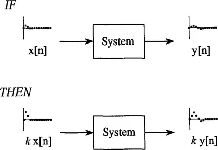
As illustrated in Fig. 5-2, homogeneity means that a change in the input signal’s amplitude results in a corresponding change in the output signal’s amplitude. In mathematical terms, if an input signal of x[n] results in an output signal of y[n], an input of kx[n] results in an output of ky[n], for any input signal and constant, k.
FIGURE 5-2 Definition of homogeneity. A system is said to be homogeneous if an amplitude change in the input results in an identical amplitude change in the output. That is, if x[n] results in y[n], then kx[n] results in ky[n], for any signal, x[n], and any constant, k.
A simple resistor provides a good example of both homogenous and non-homogeneous systems. If the input to the system is the voltage across the resistor, v(t), and the output from the system is the current through the resistor, i(t), the system is homogeneous. Ohm’s law guarantees this; if the voltage is increased or decreased, there will be a corresponding increase or decrease in the current. Now, consider another system where the input signal is the voltage across the resistor, v(t), but the output signal is the power being dissipated in the resistor, p(t). Since power is proportional to the square of the voltage, if the input signal is increased by a factor of two, the output signal is increased by a factor of four. This system is not homogeneous and therefore cannot be linear.
The property of additivity is illustrated in Fig. 5-3. Consider a ...