Singular Optics

Gregory J. Gbur

• Éditeur: CRC Press
• Année: 2016
• ISBN:
  9781315356686
• Édition: 1
• Sujet: Mathématiques
• Sous-sujet: Arithmétique

"This engagingly written text provides a useful pedagogical introduction to an extensive class of geometrical phenomena in the optics of polarization and phase, including simple explanations of much of the underlying mathematics." —Michael Berry, University of Bristol, UK

"The author covers a vast number of topics in great detail, with a unifying mathematical treatment. It will be a useful reference for both beginners and experts…." —Enrique Galvez, Charles A. Dana Professor of Physics and Astronomy, Colgate University

"a firm and comprehensive grounding both for those looking to acquaint themselves with the field and those of us that need reminding of the things we thought we knew, but hitherto did not understand: an essential point of reference." —Miles Padgett, Kelvin Chair of Natural Philosophy and Vice Principal (Research), University of Glasgow

This book focuses on the various forms of wavefield singularities, including optical vortices and polarization singularities, as well as orbital angular momentum and associated applications. It highlights how an understanding of singular optics provides a completely different way to look at light. Whereas traditional optics focuses on the shape and structure of the non-zero portions of the wavefield, singular optics describes a wave's properties from its null regions. The contents cover the three main areas of the field: the study of generic features of wavefields, determination of unusual properties of vortices and wavefields that contain singularities, and practical applications of vortices and other singularities.

CHAPTER 1

Introduction

Vortices in Nature

IT HAS LONG BEEN said that “Nature abhors a vacuum.” This statement, the sense of which was first attributed to Aristotle, is in fact oversimplified and not really true, given that most of the universe is essentially an empty space. However, even if nature abhors a vacuum, it absolutely loves a vortex.

Vortices—circulating disturbances of an extended medium of some sort of “stuff”—are quite ubiquitous in nature. They can be found on extremely small scales, in quantum mechanical Bose–Einstein condensates, on terrestrial scales in turbulent liquids and gases, and even on cosmological scales in the swirling of spiral galaxies. We now know that they are readily found in light, as well, and an investigation into the properties of such optical vortices and related structures forms the bulk of this book. The field of study of vortices and other optical singularities is now known as singular optics; we will elaborate on the meaning of “singular” in this context momentarily.

What sort of behaviors do we expect a vortex of light to have? We can actually learn much about optical vortices by looking at early studies of their liquid and gas counterparts; we will learn even more from looking at their differences.

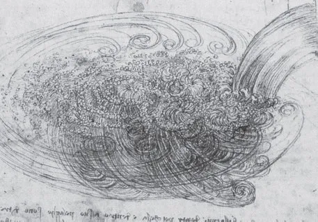
One of the earliest technical drawings of a collection of vortices was produced by the famed Leonardo da Vinci (1452–1519), in his “Studies of water passing obstacles and falling,” shown in Figure 1.1. Water falling into a pond produces an area of turbulence, and on either side of this area, we see the development of regions of opposing circulation. This already is comparable to something we will see again and again in the optical regime: the production of vortices in pairs of opposite handedness. This water example is roughly analogous to light propagation through an aperture with a size comparable to the wavelength, as will be discussed in Chapter 8. We might have predicted this pair production from conservation of angular momentum: the water entering the pond has no net circulation, so, there must also be no net circulation introduced into the water of the pond itself. In Chapter 5, we will see that vortices of light also typically have angular momentum associated with them.

FIGURE 1.1 Detail from Leonardo da Vinci’s “Studies of water passing obstacles and falling,” c. 1508.

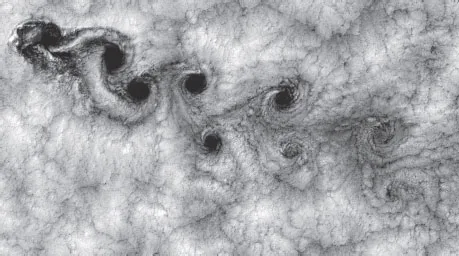
Vortex production is also quite common in the atmosphere, most strikingly in the production of the so-called von Karman vortex streets. When fluid flows around a blunt rigid obstacle at a sufficient speed, it can break up into vortices of alternating handedness that are then carried downstream, as shown in Figure 1.2. At low flow rates, pairs of vortices are produced in the “shadow” of the obstacle; when the flow becomes sufficiently high, it can peel off individual vortices from this shadow, providing enough kick to release the next vortex, and thus repeating the pattern. This vortex kick actually induces a force on the obstacle, potentially making it vibrate, and in recent years, this vortex-induced vibration (VIV) has been proposed as a new hydroelectric energy source [BRBSG08]. The vortices persist even after being released from the obstacle that created them; we will see that optical vortices are also robust structures in optical waves, making them useful for applications such as free-space optical communications, as discussed in Chapter 6.

FIGURE 1.2 Landsat 7 image of clouds near the Juan Fernandez Islands on September 15, 1999. The von Karman streets are formed by the airflow around the mountains on the islands in the upper left.

Another dramatic example of vortex creation in the atmosphere is the wingtip vortices created by airplanes. Roughly speaking, an airplane develops lift because the air flows faster over the top of the wing than the bottom of the wing, resulting in an upward Bernoulli force. This imbalance of air speeds also results in a net circulation of air around the wing, which manifests as an air vortex on the wingtip, as seen in Figure 1.3. Curiously, it is also possible to make a microscopic wing that can fly on a beam of light, as shown by Swartzlander et al. [SPAGR10]; we will touch upon this research in Chapter 5.

In fluids, then, it turns out that vortices are a surprisingly common phenomenon, which will often manifest without any deliberate experimental steps needed to be taken. In the study of singularities, we will refer to structures that appear “naturally” under “typical” circumstances as generic, and the generic properties of optical vortices will be studied in detail in Chapter 3.

FIGURE 1.3 Wingtip vortex of passing aircraft visible in smoke, from a wake vortex study on Wallops Island. (Image taken in 1990 by NASA Langley Research Center.)

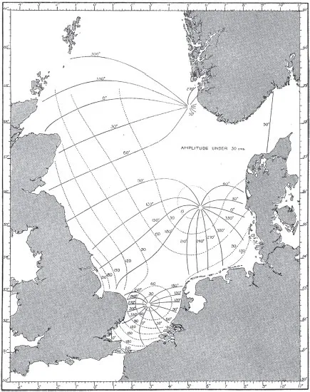
The fluid vortices mentioned so far, however, involve a transport of matter. In Da Vinci’s water vortices, for instance, actual water molecules are moving in circular paths around the vortex center. What we are really interested in, however, are wave vortices, in which it is a wave that circulates around a central point. Such wave vortices can also appear in water, and we can use monochromatic (single frequency) water wave vortices to better understand their analogous relatives in optical fields. In the beginning of the twentieth century, Proudman and Doodson [PD24] calculated the daily tidal elevations of the North Sea from a set of observational data, building upon earlier work by Whewell [Whe33]. Their map of the cotidal lines and corange lines are shown in Figure 1.4.

The cotidal lines represent the lines of high tide at different times of the day, while the corange lines represent the relative amplitudes of those tides. We can clearly see that all the cotidal lines converge together at several points known as amphidromic points, where the amplitude of the tides simultaneously goes to zero. This means that there are no tidal variations at all at the amphidromic points, which is the only possible outcome at a location where all the high-tide lines join. These points are singularities of the cotidal lines, the latter of which are equivalent to the surfaces of constant phase of an optical wavefield. As a 12-hour cycle passes, the lines of high tide circulate around the singularities, much like the hour hand of a clock moves around its central axis. This constant circulation of the tides around the amphidromic points justifies our use of the word “vortex” to describe such points. Unlike the earlier vortex examples, however, it should be noted that there is no physical transport of water around the tidal vortices: only energy and momentum circulate around the vortex.

FIGURE 1.4 Map of cotidal (solid) and corange (dashed) lines of tides in the North Sea. (From J. Proudman and A.T. Doodson. Phil. Trans. Roy. Soc. Lond. A, 224:185–219, 1924.)

It should be further noted that, following a path on the map around one of the amphidromic points, the phase of the tides increases or decreases by 360 degrees (2π radians). The periodicity of the tides (which repeat after 12 hours) and the continuity of them (there can be no discontinuous “jump” of the tide heights) implies that the phase increase or decrease around an amphidromic point must always be a multiple of 2π. From the figure, however, we note that it seems that only increases of 2π are common, or generic, to use the term introduced above. The connection between the tides and phase singularities was discussed in detail by Nye, Hajnal, and Hannay [NHH88].

But what about phase singularities in light fields? In this book, we will investigate the properties of complex scalar monochromatic wavefields u(r) that are a function of position r = (x, y, z). Such complex fields may be expressed in terms of their real and imaginary parts, the real-valued functions u_R(r) and u_I(r), in the form

$u\left(r\right)=u_R\left(r\right)+i{u}_I\left(r\right).$

(1.1)

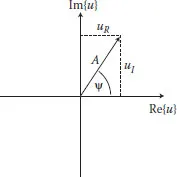
The value of such a field at any position r may be represented by a point in the complex u_R, u_I plane. However, we may also write this complex function u(r) in a polar representation in terms of a real amplitude A(r) and real phase ψ(r),

$u\left(r\right)=A\left(r\right)e^{i\text{ψ}\left(r\right)}.$

(1.2)

The relation between the Cartesian and polar representations of a complex field is illustrated in Figure 1.5. We immediately note that a zero of the field, that is, u(r) = 0, implies that A(r) = 0 and that ψ(r) is consequently undefined, that is, singular: any value of ψ(r) is valid at such points. Regions of space where a field has zero amplitude are therefore referred to as phase singularities.

FIGURE 1.5 Representation of a complex scalar field in the complex plane in Cartesian and polar forms.

The singular nature of ψ(r) at a point where A(r) = 0 would at first glance appear to be a mathematical oddity, only significant because of our preference for working in a polar representation. If we look at the phase structure of the field around such singular points, however, we can see that much more is going on! In Figure 1.6, we illustrate the phase and intensity contours of a sum of four arbitrarily chosen plane waves. We will not concern ourselves with the details of the calculations at this point, but note that the phase contours include multiple points where all lines of constant phase conv...