Simulation and Control of Chaotic Nonequilibrium Systems

With a Foreword by Julien Clinton Sprott

William Graham Hoover, Carol Griswold Hoover

• Éditeur: WSPC
• Année: 2015
• ISBN:
  9789814656849
• Sujet: Naturwissenschaften
• Sous-sujet: Thermodynamik

This book aims to provide a lively working knowledge of the thermodynamic control of microscopic simulations, while summarizing the historical development of the subject, along with some personal reminiscences. Many computational examples are described so that they are well-suited to learning by doing. The contents enhance the current understanding of the reversibility paradox and are accessible to advanced undergraduates and researchers in physics, computation, and irreversible thermodynamics.

Request Inspection Copy

Contents:

• Overview of Atomistic Mechanics
• Formulating Atomistic Simulations
• Thermodynamics, Statistical Mechanics, and Temperature
• Continuum Mechanics: Continuity, Stress, Heat Flux, Applications
• Numerical Molecular Dynamics and Chaos
• Time-Reversible Atomistic Thermostats
• Key Results from Nonequilibrium Simulations
• Second Law, Reversibility, Instability
• Outlook for Progress and Life on Earth

Readership: Advanced undergraduates and researchers in physics, computation and irreversible thermodynamics.
Key Features:

• Provides both a comprehensive historical background and contemporary research ideas and results in a variety of fields: computational simulation of irreversible flows, thermodynamics, chaos and instability, control theory
• Readers can replicate and generalize the many illustrative problems detailed in the book

Chapter 1

An Overview of Atomistic Mechanics

Topics

Many-Body Mechanics / Controlling Mechanical Boundaries / Controlling Thermal Boundaries / Gibbs’ Statistical Mechanics / Nosé-Hoover Temperature Control / Nonequilibrium Multifractal Distributions / Nonlinear Transport / Time-Reversible Thermostats and Thermometers / Background for Our Numerical Examples /

1.1Newton’s, Lagrange’s, and Hamilton’s Mechanics

Most of classical mechanics is devoted to the evolution of isolated systems with conserved energies. In this book we develop generalized versions of mechanics describing “open” systems, systems where work is done by external forces and heat is exchanged with external reservoirs. Classical mechanics, Newtonian, Lagrangian, and Hamiltonian, is the natural place to start. To begin we review the structure of Newton’s 17th century approach to the subject. Newton’s mechanics describes the time evolution of the coordinates {x(t), y(t), z(t)} defining the system of interest. These coordinates may change with the time t. The natural method for dealing with such changes is the calculus of differential equations. Newton invented (or discovered) calculus in order to treat the rates of change of coordinates in a quantitative way.

The first time derivatives of the coordinates define the “velocity” υ =

, a vector with as many components as there are coordinates:{υ_x, υ_y, υ_z}.

We will often use a superior dot shorthand “^.” to indicate a “comoving” time derivative, a time derivative following the motion. The second time derivative of each coordinate defines the corresponding acceleration a:

Newton’s Second Law relates particles’ accelerations to their masses {m} and to the forces imposed upon those masses:

Newton’s First Law describes the special case F ≡ 0 and his Third “action-reaction” Law we will often set out to violate. The Second Law is useful.

Given initial values of all the coordinates and velocities and a recipe for the forces {F} giving the accelerations we can integrate the motion equations,

into the future (or into the past) to find the particle trajectories {x(t), y(t), z(t)}. Usually the forces in classical mechanics depend only on coordinates. In our generalizations we will often use forces which depend on velocities as well as coordinates.

Gravitational forces are proportional to particle mass and provide accelerations inversely proportional to the square of the separation:

F_r = ma_r = m(d/dt)υ_r ∝ −m/r².

Likewise, electrical forces are proportional to particle charge, providing a second source for inverse-square forces. Both these results are empirical. Newton reasoned that the accelerations—the second time derivatives of the coordinates—are the fundamental mechanism for change. His First Law of Motion states that in the absence of a force (or acceleration) the velocity proceeds unchanged. It follows that x,

, and

are enough to generate the entire history and future for x(t). Separate laws for

, and higherderivatives are unnecessary. Newton had in mind that the gravitational attractive forces felt by apples and stars were proportional to the masses of the interacting bodies and inversely proportional to the inverse square of their separation. It is interesting that this inverse-square “law” is specific to three-dimensional space. In two dimensions the corresponding force is −(m₁m₂/r₁₂) rather than

.

For instance, a two-dimensional particle with coordinates (x, y) and unit mass, attracted to the origin by an attractive force (−1/r), satisfies conservation of (kinetic plus potential) energy,

:

Because the x and y terms separately cancel a linear combination (corresponding to an ellipse) also satisfies the conservation of energy. In a “conservative” system, with constant total energy E = K(v) + Φ(r), the change of kinetic energy with time compensates that due to the changing potential,

.

“Generalized coordinates” {q} (angles are the most common case) and their conjugate momenta {p}, can be treated with Lagrangian mechanics where the Lagrangian is the difference,

, between the kinetic and potential energies. Lagrange’s equations of motion define the momenta and their time-rates-of-change:

In the Cartesian case with K(

) and Φ(q) Lagrange’s motion equations reproduce Newton’s. Lagrange’s equations generalize Newton’s approach to systems with curvilinear coordinates and also facilitate the inclusion of constraints (fixed bond lengths, fixed kinetic energies, …).

Hamilton’s equations of motion are a particularly useful additional generalization of Newton’s approach. In Newtonian and Lagrangian mechanics accelerations depend upon the second derivatives of the coodinates. In Hamiltonian mechanics the coordinates {q} and momenta {p} are independent variables. Their time development is governed by Hamilton’s first-order equations of motion,

The underlying Hamiltonian is typically the sum of the kinetic and potential energies,

. The Hamiltonian is also basic to quantum mechanics.

For us the most important consequence of Hamiltonian mechanics is Liouville’s Theorem. In classical mechanics the Theorem states that the comoving “phase volume” is unchanged by the motion equations:

Here # is the number of “degrees of freedom”. Each degree of freedom q and its corresponding momentum p together represent two independent phase-space coordinates. The theorem is easy to prove. We will go through all of the details in Section 2.3, and show that flows in phase space, described by Hamilton’s equations of motion, obey a many-dimensional analog of the continuum continuity equation for an incompressible fluid:

In quantum mechanics, the momentum in the classical Hamiltonian is replaced by a differential operator p → iħ(∂/∂q) = i(h/2π)(∂/∂q), in Schrödinger’s stationary-state equation

ψ = Eψ for the wave function ψ corresponding to the energy E.h is Planck’s constant.

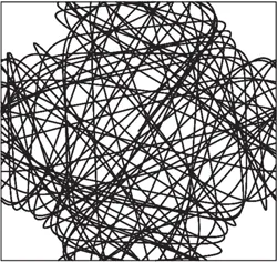
The classical motion equations are either first-order or second-order ordinary differential equations and can be solved with a variety of numerical methods. Despite this simple structure, applications of the equations can produce complicated results, even for a one-body problem, as we show in the following Section. Around 1900 Poincaré recognized what is now called chaos, or the (exponential) sensitivity of results to initial conditions. Chaos can be present even in the one-body problem, as we shall soon see.

Fig. 1.1 Cell model dynamics. A single particle is accelerated by four fixed “scatterers”.

1.2Controlling Mechanical Boundaries

Most applications of mechanics take place within a fixed region in space. The one-dimensional harmonic oscillator has a periodic solution near the coordinate origin, x ∝ cos(ωt), where the frequency ω = 2πν depends on the force constant and the mass of the oscillator. A zero-pressure solid or fluid with fixed center of mass has no tendency to explore its surroundings, instead just vibrating and/or rotating as time goes on. Many-body systems can be confined in a rigid container but show much less number dependence in their properties if periodic boundaries are used.

Figure 1.1 illust...