Output Expenditure Model

7 Key excerpts on "Output Expenditure Model"

• 

  eBook - PDF

  21st Century Economics: A Reference Handbook

  • Rhona C. Free(Author)
  • 2010(Publication Date)
  • SAGE Publications, Inc

    (Publisher)

  31 AGGREGATE EXPENDITURES MODEL AND EQUILIBRIUM OUTPUT MICHAEL R. MONTGOMERY University of Maine A ggregate expenditures (AE), the total spending in an economy on final goods and services over a designated time period, is the core demand-side concept in modern macroeconomics (a final good is a newly produced good bought by a user who will finally dispose of that good by using up its services). Following the lead of John Maynard Keynes in his General Theory of Employment, Interest and Money (1936/1965) and early Keynesians such as Alvin Hansen (1953) and Paul A. Samuelson (1939), AE is typically broken down by major type of purchaser into consumption expenditures, invest-ment expenditures, government expenditures, and the sum of exports less imports (known as net exports). The study of these categories in recent decades has been aided con-siderably by the development of the National Income and Product Accounts (NIRA) accounting system, which is used by governments in measuring and reporting the sizes of these categories. The sum of this spending is known as gross domestic product, or GDP. Specifically, • Consumption expenditures are expenditures on final goods (excluding housing) and services by consumers, produced during the accounting period and in the economy under study. • Investment expenditures are final goods and services purchased by businesses and buyers of homes, produced during the accounting period and in the economy under study. They include nonresidential structures of all types, plus all producers' durable equipment, plus residential structures, plus all inventories produced in the accounting period (some of these inventories may be planned, or desired, inventories; others may be unplanned, or undesired, inventories—unplanned inventories being acquired when sales are less than anticipated). Investment expenditures do not include financial transactions such as the purchase of stocks and bonds.

  Sign up to read

  Learn more about book
• 

  eBook - PDF

  Economics

  • William Boyes, Michael Melvin(Authors)
  • 2015(Publication Date)
  • Cengage Learning EMEA

    (Publisher)

  It is called the Keynesian model . This model of the economy can be very useful in explaining some real-world events, but it suffers from a serious drawback: It assumes that the supply of goods and services in the economy always adjusts to aggregate expen-ditures, that there is no need for price changes. The Keynesian model is a fixed-price model . In the real world, we find that shortages of goods and services are often met by rising prices, not just increased production. We also find that when supply increases in the face of R E C A P 1. Any change in autonomous expenditures is multiplied into a larger change in the equilib-rium level of real GDP. 2. The multiplier measures the change in equilibrium real GDP produced by a change in autonomous spending. 3. The multiplier equals 1 Leakages ¼ 1 MPS þ MPI 4. The recessionary gap is the amount by which spending must increase in order to achieve equilibrium at potential real GDP. Graphically, it is measured by the vertical distance between the 45-degree line and the aggregate expenditures curve at potential real GDP. 5. The true spending multiplier may differ from the simple spending multiplier (1/[ MPS þ MPI ]) because of the foreign repercussions of domestic spending. Price changes and taxes cause the simple spending multiplier to overestimate the true multiplier. Chapter 10 Income and Expenditures Equilibrium 217 Copyright 2016 Cengage Learning. All Rights Reserved. May not be copied, scanned, or duplicated, in whole or in part. Due to electronic rights, some third party content may be suppressed from the eBook and/or eChapter(s). Editorial review has deemed that any suppressed content does not materially affect the overall learning experience. Cengage Learning reserves the right to remove additional content at any time if subsequent rights restrictions require it. relatively constant demand, prices may fall. In other words, prices as well as production adjust to differences between demand and supply.

  Sign up to read

  Learn more about book
• 

  eBook - ePub

  Economics for Investment Decision Makers

  Micro, Macro, and International Economics

  • Christopher D. Piros, Jerald E. Pinto(Authors)
  • 2013(Publication Date)
  • Wiley

    (Publisher)

  Profit is the return that owners of a company receive for the use of their capital and the assumption of financial risk when making their investments. Although businesses are the direct owners of much of the property and physical capital in the economy by virtue of owning the businesses, households are the ultimate owners of these assets and hence the ultimate recipients of the profits. In reality, of course, a portion of profits is usually retained within businesses to help finance maintenance and expansion of capacity. Similarly, because the government is viewed as operating on a nonprofit basis, any revenue it receives from ownership of companies or property may be viewed as being passed back to households in the form of lower taxes. Therefore, for simplicity, it is standard in macroeconomics to attribute all income to the household sector unless the analysis depends on a more precise accounting.

  Aggregate expenditure , the total amount spent on the goods and services produced in the (domestic) economy during the period, must also be equal to aggregate output and aggregate income. However, some of this expenditure may come from foreigners in the form of net exports.1 Thus, aggregate output, aggregate income, and aggregate expenditure all refer to different ways of decomposing the same quantity.

  Exhibit 5-1 illustrates the flow of inputs, outputs, income, and expenditures in a very simple economy. Households supply the factors of production (labor and capital) to businesses in exchange for wages and profit (aggregate income) totaling £100. These flows are shown by the top two arrows. Companies use the inputs to produce goods and services (aggregate output), which they sell to households (aggregate expenditure) for £100. The output and expenditure flows are shown by the bottom two arrows. Aggregate output, income, and expenditure are all equal to £100.

  EXHIBIT 5-1 Output, Income, and Expenditure in a Simple Economy: The Circular Flow

  In this simplified example, households spend all of their income on domestically produced goods and services. They do not buy foreign goods, save for the future, or pay taxes. Similarly, businesses do not sell to foreigners or to the government and do not invest to increase their productive capacity. These important components of the economy will be added in Section 2.2. But first we need to discuss how output and income are measured.

  Sign up to read

  Learn more about book
• 

  eBook - PDF

  Macroeconomic Modelling

  • S.G. Hall, S.G.B. Henry(Authors)
  • 2014(Publication Date)
  • North Holland

    (Publisher)

  It is often thought of as the implementation of conventional Keynesian theoretical views. In this model the assumption is generally made that the demand side of the model is dominant, so that X = X D . The supply side of many of the markets are then virtually ignored, and prices are set on a fairly f ad hoc 1 cost mark up basis. To be more specific, total output in such a model is generally determined by total demand which, in turn, is determined by summing the components of aggregate expenditures, consumption, investment, stockbuilding, etc. The central, expenditure, part of the model then determines the real components of the economy, and it is around this central structure that additional sectors determining prices and monetary aggregates may be added. Most of the large forecasting models follow this general structure and although the largest may involve several thousand variables the conceptual approach is common. Other classes of models include equilibrium models, supply-side models, disequilibrium models and bargaining models. All of these may, at least in part, be seen as attempts to relax the restrictive assumption of demand side dominance of the income expenditure model, and to cope with the question of how prices are actually determined within the system. 1 32 Ch. 4: Macro Models 133 An equilibrium model, for example, makes the general assumption that markets continuously clear so X = X * X , and prices are set so that market clearing occurs. In order to deal with the regular fluctuations which actually occur in real variables, such models often distinguish between the actual value of a variable and its equilibrium value, and simply postulate that the two come together quickly. While the assumption of continuous market clearing may be viewed as an extreme one, a major advantage of this approach is that it does offer a sound theoretical foundation for the determination of prices within the model.

  Sign up to read

  Learn more about book
• 

  eBook - PDF

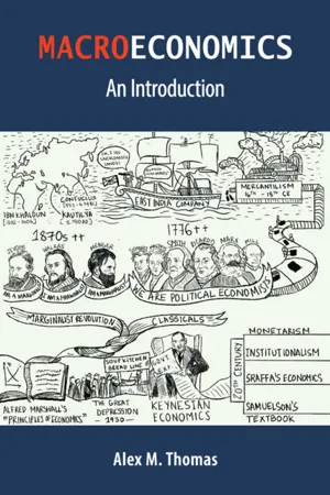
  Macroeconomics

  An Introduction

  • Alex M. Thomas(Author)
  • 2021(Publication Date)
  • Cambridge University Press

    (Publisher)

  The precise value of the government expenditure multiplier can be obtained by dividing the change in aggregate output (ΔY) by the change in government expenditure (ΔG), ceteris paribus. Suppose now that the value of the government expenditure multiplier (ΔY/ΔG) is greater than the consumption expenditure multiplier (ΔY/ΔC) and further suppose that your aim is to increase employment. Would you devote additional resources to G or to C? And besides increasing employment, what are the other socioeconomic purposes of consumption and government expenditure? Underlying the concept of the multiplier is the meso or structural approach to economics. In Figure 2.2, focus on the flows between the government and the non-f inancial sector. The expenditure of the government on the goods and services of the non-f inancial sector provides the non-f inancial sector with an income, in addition to that arising from the expenditure of the household sector. However, the additional government expenditure is not a one-off flow because it generates additional income that can generate additional employment, which further leads to additional income and additional expenditure by the household sector, so on and so forth. The value of the multiplier captures all the direct and indirect effects on aggregate output. And to understand what is happening within the black box of the non-financial sector in Figure 2.2, look at Table 2.1, which gives us an idea of the interrelationship within the non-financial sector in terms of the structural interdependence between the primary, secondary and tertiary sectors. Additional incomes are also generated within the non-f inancial sector. Thus, in macroeconomics, the understanding that expenditure generates income is pivotal. OUTPUT AND eMPLOYMeNT LeVeLS 77 Autonomous and induced elements of aggregate demand Now, let me introduce you to the conceptual distinction between autonomous and induced elements of aggregate demand.

  Sign up to read

  Learn more about book
• 

  eBook - ePub

  Financial Programming and Policy : The Case of Sri Lanka

  • John Karlik, Michael Bell, M. Martin, S. Rajcoomar, and Charles Sisson(Authors)
  • 1996(Publication Date)
  • INTERNATIONAL MONETARY FUND

    (Publisher)

  IV. Output, Expenditure, and Prices

  Passage contains an image

  1. Introduction

  The ultimate objective of financial programming is to establish an economic framework for sustainable growth. This goal cannot be achieved without a realistic forecast of output, expenditure, and prices in the program period. The forecast serves as the basis for subsequent sectoral projections of the fiscal, monetary, and balance of payments accounts. This section, then, discusses the conceptual framework for determining output, expenditure, and prices and suggests some practical projection techniques. During the financial programming exercise at the end of the workshops, a consistency check is conducted to ensure that projections for the budgetary, monetary, and balance of payments accounts forecasting workshops are consistent with the initial projections established in this workshop.

  Passage contains an image

  2. Determining Output: A Conceptual Framework

  a. Potential vs. actual output

  Targeting the real growth in output is one of the most important elements of a financial program. To be credible, the output target has to be compatible not only with the other elements of a program but also with external realities and the special features of the domestic economy.

  The level of output produced in a given period is a function not only of the inputs used during the production process but also of the way they are used and includes technological, managerial, and environmental factors. Thus, output depends in part on how efficiently inputs are combined, and the volume of the inputs themselves is a function of past output. In industrial countries in particular, these relationships are often analyzed using an aggregate production function that indicates the relationship between output and inputs, or factors of production. This function can be written as follows:

  Sign up to read

  Learn more about book
• 

  eBook - ePub

  International Economics (Routledge Revivals)

  • David Gowland(Author)
  • 2010(Publication Date)
  • Taylor & Francis

    (Publisher)

  As the absorption approach is the open economy version of the Keynesian model, this is usually illustrated by an analysis in which output is demand-determined. In this case output is X+(1−m) (C+I+G), where m is the marginal propensity to import, i.e. output is that which is necessary to satisfy export demand plus the part of home demand not spent on imports. In this case the fall in output is (1−m) times the fall in expenditure; exports are taken to be exogenous. This fall in output is obviously less than the fall in expenditure (unless m is negative). The improvement in the balance of payments is m times (the fall in expenditure). In effect, a reduction in (C+I+G) automatically reduces imports and so improves the balance of payments. This conclusion is perhaps obvious and the analysis simplistic, but like so many other obvious facts, it took economists to point it out! (In such models, it is necessary for m to be less than 1 otherwise the model is unstable; this is not demonstrated as the model is only illustrative and it is difficult to see how m could exceed 1, so long as other influences are properly specified.) The next statements, (2) and (3) above, are very easy to demonstrate. So long as output is fixed, an improvement in the balance of payments must be accompanied by a reduction in expenditure. Even if output can rise, it is necessary to ensure that output rises by more than expenditure. In both cases, any impact of a devaluation will be negated by income effects—as in the example in Chapter 6 —unless expenditure is controlled by deflationary policies. Absorption analysis can be used to demonstrate this formally and to put into the appropriate framework statements made at a more elementary level. This is not its sole merit as it is a very flexible framework into which almost any analysis can be put. One of the most common and useful involves the concepts of ‘expenditure switching’ and ‘expenditure reducing’

  Sign up to read

  Learn more about book