Mathematics
Coordinate Geometry
Coordinate geometry is a branch of mathematics that combines algebra and geometry. It involves studying geometric figures using coordinates and equations. By representing points, lines, and shapes on a coordinate plane, it allows for the application of algebraic techniques to solve geometric problems.
Written by Perlego with AI-assistance
Related key terms
1 of 5
12 Key excerpts on "Coordinate Geometry"
 eBook - PDF
- D.H. Maling(Author)
- 2013(Publication Date)
- Pergamon(Publisher)
The branch of mathematics known as Coordinate Geometry analyses problems through the relationship between points as defined by their coordinates. By these means, for example, it is possible to derive algebraic expressions defining different kinds of curve which cannot be done by Euclidean geometry. Coordinate Geometry is an exceptionally powerful tool in the study of the theory of map projections, and without its help it is practically impossible to pass beyond the elementary descrip-tive stage. Plane Coordinate Geometry is usually studied first through the 27 28 Coordinate Systems and M a p Projections medium of the conic sections or the definition of the different kinds of curve formed by the surface of a cone where this has been intersected by a plane. Two of the resulting sections, the ellipse and the circle, are of fundamental importance to the theory of distortions in map projections. There are an infinite number of ways in which one point on a plane surface may be referred to another point on the same plane. Every map projection creates a unique reference system which satisfies this requirement and an infinity of different map projections could theo-retically be described. However it is desirable to use some kind of coor-dinate system to describe, analyse and construct each of these projections. Any system to be used for such purposes ought to be easy to understand and simple to express algebraically. For plane representation the choice lies between plane cartesian coordinates and polar coordinates. Plane cartesian coordinates The reader will already be familiar with graphs as a method of plotting two variables on specially ruled paper and with the National Grid on Ordnance Survey maps. The graph and the National Grid are simple, but special, examples of plane cartesian coordinates. In the general case, any plane coordinate system which makes use of linear measurements in two directions from a pair of fixed axes can be regarded as a cartesian system. eBook - PDF
Mathematics for Elementary Teachers
A Contemporary Approach
- Gary L. Musser, Blake E. Peterson, William F. Burger(Authors)
- 2013(Publication Date)
- Wiley(Publisher)
AUTHOR WALK-THROUGH 782 INTRODUCTION In this chapter we study geometry using the coordinate plane. Using a coordinate system on the plane, which was introduced in Section 9.4, we are able to derive many elegant geometric results about lines, polygons, circles, and so on. One of the benefits of studying geometry on a coordinate system is the relationship with algebraic ideas. This can help prospective teachers understand geometric ideas because of their experience in algebra classes. When children investigate geometry on a coordinate system, it can lay a foundation for studying algebra in the future. In Section 15.1, we introduce the basic ideas needed to study geometry in the coordinate plane. Then in Section 15.2 we prove properties of geometric shapes using these concepts. Finally, Section 15.3 contains many interesting problems that can be solved using coor- dinate geometry. Key Concepts from the NCTM Principles and Standards for School Mathematics GRADES PRE-K-2–GEOMETRY Describe, name, and interpret relative positions in space and apply ideas about relative position. Find and name locations with simple relationships such as “near to” and in coordinate systems such as maps. GRADES 3-5–GEOMETRY Describe location and movement using common language and geometric vocabulary. Make and use coordinate systems to specify locations and to describe paths. Find the distance between points along horizontal and vertical lines of a coordinate system. GRADES 6-8–GEOMETRY Use Coordinate Geometry to represent and examine the properties of geometric shapes. Use Coordinate Geometry to examine special geometric shapes, such as regular polygons or those with pairs of parallel or perpendicular sides. Key Concepts from the NCTM Curriculum Focal Points GRADE 3: Describing and analyzing properties of two-dimensional shapes. GRADE 6: Writing, interpreting, and using mathematical expressions and equations.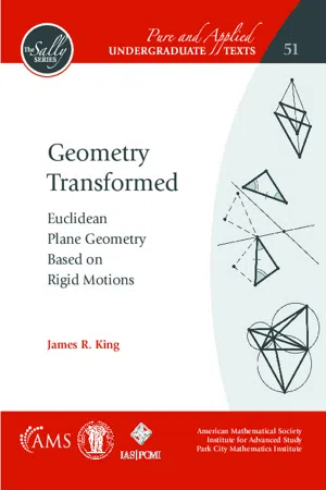 eBook - PDF
Geometry Transformed
Euclidean Plane Geometry Based on Rigid Motions
- James R. King(Author)
- 2021(Publication Date)
- American Mathematical Society(Publisher)
Chapter 11 Coordinate Geometry Coordinates attach numbers to points in such a way that algebra can be used to inves-tigate geometry. In the 17th century, Fermat and Descartes developed the beginnings of the coordinate systems that are so familiar today. To express rigid motions and distance and angle relationships, we will want a Cartesian coordinate system with perpendicular axes and rulers on each axis. But there are applications that do not require such a restricted coordinate system, so we begin more simply with parallel lines and ratios to define what are called affine or linear coordinates. Then we develop formulas for half-turns and translations and equations for lines in affine coordinates. Afterwards, for the metric part of Euclidean geometry, we will restrict ourselves to Cartesian coordinates, which are coordinates with more constraints on angles and distances. The introduction of coordinates will connect the abstract model of the plane de-veloped up to now with algebra and the (?, ?) -plane ℝ 2 . This will provide some new algebraic tools for studying geometry, but the geometry will also provide insight into the algebra. Axes and Coordinates In the plane, take a triangle △? 0 ? 1 ? 2 as the reference triangle for a system of coordi-nates based on parallel lines and signed ratios. On the line ? 0 ? 1 , let ?(?) = ? 0 ?/? 0 ? 1 . This ratio is a coordinate proportional to a ruler on the line, with ?(? 0 ) = 0 and ?(? 1 ) = 1 . In the same way, on ? 0 ? 2 , let ?(?) = ? 0 ?/? 0 ? 2 . The first axis, or ? -axis , of the coordinate system is ? 0 ? 1 ; the second axis, or ? -axis , is ? 0 ? 2 . The origin of the system is the point ? 0 . For any point ? in the plane, let ? 1 be the line through ? parallel to or equal to the ? -axis. This line intersects the ? -axis at a point ? 1 . Define ?(?) = ?(? 1 ) . 217 218 11. Coordinate Geometry E 0 P 1 E 0 E 1 = 3.00 E 0 P 2 E 0 E 2 = 2.00 P 1 P 2 P (3,2) Q (-1, .5) E 0 E 1 E 2 Figure 1. eBook - PDF
- Daniel C. Alexander, Geralyn M. Koeberlein(Authors)
- 2019(Publication Date)
- Cengage Learning EMEA(Publisher)
(See Appendices A.2 and A.3 for further information.) In much of this chapter, we deal with equations containing two variables; to relate such alge- braic statements to plane geometry, we will need two number lines. The study of the relationships between number pairs and points is known as analytic geometry. The Cartesian coordinate system or rectangular coordinate system is the plane that results when two number lines intersect perpendicularly at the origin (the point corresponding to the number 0 of each line). This two-dimensional coordinate plane is often called the Cartesian plane, named in honor of René Descartes (see Perspective on History for Chapter 9). The horizontal number line is known as the x-axis, and its numer- ical coordinates increase from left to right. On the vertical number line, the y-axis, values increase from bottom to top; see Figure 10.1. The scale (unit size) is generally the same for the x-axis and the y-axis. The two axes separate the plane into four quadrants, which are numbered counterclockwise I, II, III, and IV, as shown. The point that marks the com- mon origin of the two number lines is the origin of the rectangular coordinate system. It is convenient to identify the origin as (0, 0); this notation indicates that the x-coordinate (listed first) is 0 and also that the y-coordinate (listed second) is 0. In the coordinate system, each point has the order (x, y) and is called an ordered pair. In Figure 10.2, the point (3, 22), for which x 5 3 and y 5 22, is shown. The point (3, 22) is located by moving 3 units to the right of the origin and then 2 units down from the x-axis. The dashed lines shown emphasize the reason why the grid is often called the rectangular coordinate system. The point (3, 22) is located in Quadrant IV. In Figure 10.2, ordered pairs of positive and negative signs characterize the signs of the coordinates of a point located in each quadrant.
- Zhilin Li(Author)
- 2006(Publication Date)
- CRC Press(Publisher)
29 Mathematical Background In the algorithms to be presented in the later chapters, mathematical tools at various levels are involved. To facilitate those discussions, this chapter provides some basic mathematical background. 2.1 GEOMETRIC ELEMENTS AND PARAMETERS FOR SPATIAL REPRESENTATION 2.1.1 C OORDINATE S YSTEMS To make a spatial representation possess a certain level of metric quality, a coordinate system needs to be employed. The Cartesian coordinate system is the basic system in Euclidean space and is most familiar to us. It could be three-dimensional (3-D) or 2-D. The latter is a result of the orthogonal projection of the former. A geographical coordinate system is also a fundamental system for spatial representation, consisting of longitude and latitude. A geographical coor-dinate system can be defined on a sphere (or spheroid) or on a 2-D plane. The latter is a result of a projection of the former. Such a projection is called a map projection . Polar coordinate systems are also possible but are not widely used in spatial representation. Figure 2.1 shows such systems in a 2-D plane. The Cartesian coordinate system is normally used for spatial representation at large and medium scales, and the geographical coordinate system is used for spatial representation at small and very small scales. In recent years raster systems have been in wide use. Through the history of spatial information science, there has been an almost constant debate about the nature and importance of raster (e.g., Peuquet, 1984; Maffini, 1987; Maguire et. al., 1991). The importance of working with multi-scale representation in raster was realized in the early 1980s (e.g., Monmonior, 1983). Mathematically elegant algo-rithms have been developed since the 1990s (Li, 1994; Li and Su, 1996; Su et al., 1997a, 1997b, 1998). A raster space is a discrete space. It is a result of partitioning a connected space into small pieces, but these pieces together cover the whole space contiguously. eBook - PDF
- Doug French(Author)
- 2004(Publication Date)
- Continuum(Publisher)
With computers and calculators which handle complexity so readily it is easy to generate diagrams and graphs which hide the important geometrical ideas that students have to master if they are to come to understand that complexity. It is also very easy for mathematical ideas to become lost through attempting to use too wide a range of commands within a software package or graphical calculator. A number of important teaching and learning points emerge from this chapter which has looked at the application of algebra to geometry through the key idea that a straight line or curve can be represented by an equation with reference to a system of coordinates: • Situations described in terms of coordinates or equations of curves need to be portrayed with a diagram rather than seen as a purely algebraic or numerical exercise. For most purposes it is not necessary to draw such diagrams accurately, because their purpose is to suggest a way of solving a problem or to give some idea of the magnitude of a numerical answer or the form of the equation of a curve. • Formulae for standard procedures such as finding the distance between two points or the gradient of a line should not be introduced at too early a stage. Particular procedures are often understood and remembered more readily through simple numerical examples which encapsulate the essential idea. • Locus is a valuable idea both in establishing the equations of standard curves and in solving more general problems. This requires an ability to formulate a relationship, usually involving lengths in a suitable algebraic form, then to carry out some simplification and finally to check and interpret the solution. As with all problems where algebra is used, it is important to give sufficient time and consideration to the important first stage of formulation and the last stage of checking and interpretation, rather than concentrate exclusively on the more mechanical aspects of the solution. eBook - PDF
Sixth Form Pure Mathematics
Volume 1
- C. Plumpton, W. A. Tomkys(Authors)
- 2014(Publication Date)
- Pergamon(Publisher)
CHAPTER II METHODS OF Coordinate Geometry 2.1 The Straight Line The equation of a straight line with a given gradient and through a given point was considered in Chapter I. The equation Ax+By 4-C = 0, where A, B and C are constant, is the equation of a curve with a con-stant gradient (d.y/djc = — A/B) and it is therefore the equation of a straight line. This form of the equation of a straight line includes all possible cases and it is called the general equation of a straight line. It should be noted that, if the coordinates of two of the points on the line are known, the ratios A:B:C can be determined uniquely. If A = 0, the line is parallel to the x-axis; if B = 0 the line is parallel to the j>-axis; if C = 0, the line goes through the origin. The line y = mx+c. This form of the equation of a straight line does not include the case x = constant. The gradient of the line is m, and c is the intercept on the >>-axis. The equation of the straight line through two given points. The gradient of the line joining the points A(xi, y{), Bfa, J2) is 0>2—>>i)/(*2—*i) (Fig. 11). The equation of the line is therefore X2 — X This is more conveniently written and remembered in the equivalent form y-yi = x—xx The equation (2.1) y2-yi x 2 -x! a b 33 34 SIXTH FORM PURE MATHEMATICS represents the line which passes through the points (a, 0), (0, b) on Ox and Oy respectively. The equation of any straight line not passing through O and not parallel to one of the coordinate axes can be expressed in this intercept form. +-x Fig. 11. The distance between two points whose coordinates are (*i, yi) 9 (x 2 , ^2). By Pythagoras' Theorem (Fig. 11), AB 2 = AP 2 +PB 2 ; . AB = V{(*i-*2)*+0>i->>2) 2 }. (2.2) Area. The area of a rectilinear figure can be obtained in special cases by various methods. The method illustrated below is the most convenient one when the coordinates of the vertices of the rectilinear figure are known.
- Carl D. Crane, III, Michael Griffis, Joseph Duffy(Authors)
- 2022(Publication Date)
- Cambridge University Press(Publisher)
1 Geometry of Points, Lines, and Planes . . . and then geometry will become what geometry ought to be. Mr. Querulous Ball’s “A Dynamical Parable” (1887) 1.1 Introduction Points, lines, and planes are the fundamental elements of spatial geometry. A point can be thought of as a location in 3D space, and its coordinates have units of length. A line can be considered to be an infinite collection of points defined by a direction (which is a dimensionless vector) that passes through some given point (which has units of meters). A plane is a two-dimensional set of points that can be defined, for example, by three points or by a line and one point. This chapter introduces the concept of homogeneous coordinates as applied to points, lines, and planes. The homogeneous coordinates of each will be defined together with the equation for each. The equation of a point, line, or plane will be shown to be a vector equation where any vector that satisfies that equation is a member of that point, line, or plane. 1.2 The Position Vector of a Point The position vector to a point Q 1 from a reference point O will be referred to as r 1 and can be expressed in the form r 1 = x 1 i + y 1 j + z 1 k w 1 (1.1) or r 1 w 1 = S O1 , (1.2) where S O1 = x 1 i + y 1 j + z 1 k and the components of the vector S O1 have units of length. The term w 1 is dimensionless. In Figure 1.1 it is assumed that w 1 = 1 and (x 1 , y 1 , z 1 ) are the usual Cartesian coordinates for the point Q 1 . The coordinates r of some general point Q may be expressed as 2 1 Geometry of Points, Lines, and Planes Figure 1.1 Coordinates of a point r w = S O , (1.3) where S O = x i + y j + z k. The subscript O has been introduced to signify that S O is origin dependent. Clearly, if we choose some other reference point, the actual point Q would not change. However, the coordinates (x , y , z), which determine Q, would change. The ratios x/w, y/w, and z/w are three independent scalars and, therefore, there are ∞ 3 points in space. eBook - PDF
Fundamental Maths
For Engineering and Science
- Mark Breach(Author)
- 2017(Publication Date)
- Red Globe Press(Publisher)
20 Coordinate systems What this chapter is about In this chapter you will investigate spatial relationships in a two-dimensional plane. By the end of this chapter you will be able to calculate distance and orientation in a two-dimensional plane, the areas of straight-sided figures, find the intersection of lines, and calculate parameters and formulae of circles. You will be able to change from Cartesian to polar coordinates and vice versa and to apply Pythagoras’ theorem in three dimensions. 20-01 Cartesian coordinate system applications The Cartesian coordinate system was introduced in Chapter 6 and it is now appropriate to look at some of its implications. The first is that not everyone uses it in the same way as mathematicians. In the Cartesian coordinate system the primary reference direction is the x -axis and orientation is measured anticlockwise from it. Geographers, and particularly land and engineering surveyors, use a system in which the primary direction is north and orientation, such as a compass bearing, is measured clockwise from it. Although the fundamental mathematical relationships are not affected by this difference, their applications may be. 20-02 Distance and orientation between two points Two points in a coordinate frame may be joined by a straight line. The length of that line will be the distance between the two points. The orientation of the line is measured with 209 Figure 20.1 north east α P ( E P , N P ) x -axis y -axis α P ( x P , y P ) respect to the x -direction within the Cartesian coordinate system and with respect to the north direction in the geographical frame. An application of Pythagoras’ theorem can be used to find the length of the line, and the tangent of its orientation relates the sides of the right angled triangles in Figure 20.2. eBook - PDF
A Collection of Problems in Analytical Geometry
Three-Dimensional Analytical Geometry
- D. V. Kletenik, W. J. Langford, E. A. Maxwell(Authors)
- 2016(Publication Date)
- Pergamon(Publisher)
P A R T II Three-Dimensional Analytical Geometry This page intentionally left blank C H A P T E R 6 ELEMENTARY PROBLEMS OF THREE-DIMENSIONAL ANALYTICAL GEOMETRY § 27. Rectangular Cartesian Coordinates in Three-dimensional Space A rectangular Cartesian coordinate system in three-dimen-sional space is defined when a unit of length for measuring lengths and three mutually perpendicular, concurrent axes are given, the axes being considered ordered. The point of intersection of the axes is called the coordinate origin, and the axes themselves are called the first, second, and third, coordin-ate axes. The origin is denoted by the letter O and the three axes by Ox, Oy, Oz respectively. Let M be an arbitrary point in space, and let M x , M y , Μ ζ be its projections on to the coordinate axes (Fig. 38). Then the coordinates of the point M in the given coordinate system are the numbers x = OM x , y = OM y , z = OM z where OM x is the measure on the interval OM x on the x-axis, OM y the measure of the interval OM y on the j-axis, and OM z the measure of the interval OM z on the z-axis. The number x is called the first coordinate of the point M, or its x-cgordinate, the number y the second coordinate or the j-coordinate, the number z the third coordinate or the z-coordinate. The co-ordinates are written in round brackets after the letter designat-ing the point: M{x, y, z). 3 4 THREE-DIMENSIONAL ANALYTICAL GEOMETRY The plane Oyz divides the whole space into two half-spaces, and the one which contains the positive direction of the x-axis will be referred to as the near half-space, and the other as the remote half-space. The plane Ozx similarly divides space into two half-spaces, and the one which contains the positive direction of the >>-axis is referred to as the right half-space, and the other as the left half-space. And, finally, the plane Oxy M 2 Mr M / V Fro. 38 K m W/ / / / '/> L / X / 0 2 / 1 , / ' 1 λ -Jf V / y FIG. eBook - PDF
Sixth Form Pure Mathematics
Volume 2
- C. Plumpton, W. A. Tomkys(Authors)
- 2014(Publication Date)
- Pergamon(Publisher)
CHAPTER XXI Coordinate Geometry OF THREE DIMENSIONS 21.1 The coordinate system Let ΧΟΧ', ΥΟΥ', ΖΟΖ' be three mutually perpendicular straight lines intersecting at the origin 0, (Fig. 174). These lines are called the coordinate axes and determine three mutually perpendicular planes (0 7, OZ), (OZ, OX), (OX, 0 Y) called the coordinate planes. The position of any point P in space is determined uniquely by its directed distances from these planes. Let L, M, N be the feet of the perpendiculars from P to the coordinate planes and let A, B, C be the other vertices (lying on the coordinate axes) of the cuboid with PL, PM, PN as adjacent edges (Fig. 174). Again with reference to this figure, displacements in the direction OX are defined as positive and displacements in the direction OX' as negative with similar definitions FIG. 174. 352 PURE MATHEMATICS in relation to the other coordinate axes. Then the coordinates (x, y, z) of P referred to the coordinate axes are defined as follows: x' = 0 A ( = LP) or — OA according as the displacement OA is positive or negative. y = 0B(= MP) or — OB according as the displacement OB is positive or negative. z = 0C(= NP) or — OC according as the displacement OC is positive or negative. The coordinate planes divide space into eight octants; in the octant OX YZ, x, y, and z are all positive; in the octant ΟΧ' ΥΖ', x and z are negative and y is positive, etc. The coordinate planes OYZ, OZX, OX Y are usually called the yz, zx, xy— planes respectively and the coordinate axes X'OX, Y'OY, Z'OZ, the x, y, z-axes respectively. eBook - PDF
Mathematical Practices, Mathematics for Teachers
Activities, Models, and Real-Life Examples
- Ron Larson, Robyn Silbey(Authors)
- 2014(Publication Date)
- Cengage Learning EMEA(Publisher)
Coordinate Geometry 15.1 The Coordinate Plane and Distance 15.2 The Slope of a Line 15.3 Linear Equations in Two Variables 15.4 Functions Rob Marmion/Shutterstock.com 565 5 Copyright 2014 Cengage Learning. All Rights Reserved. May not be copied, scanned, or duplicated, in whole or in part. Due to electronic rights, some third party content may be suppressed from the eBook and/or eChapter(s). Editorial review has deemed that any suppressed content does not materially affect the overall learning experience. Cengage Learning reserves the right to remove additional content at any time if subsequent rights restrictions require it. 566 Chapter 15 Coordinate Geometry Activity: Plotting Points in the Coordinate Plane Materials: • Pencil Learning Objective: Understand how to plot points in the coordinate plane, including points in all four quadrants. Name _____________________________ Plot the ordered pairs in the coordinate plane. Connect the points in numerical order. 1(1, 11) 2(−4, 9) 3(−5, 7) 4(−6, 6) 5(−6, 5) 6(−3, 2) 7(−4, 1) 8(−8, 3) 9(−9, 2) 10(−9, 1) 11(−5, −1) 12(−4, −4) 13(−5, −6) 14(−7 −5) 15(−8, −6) 16(−8, −7) 17(−4, −10) 18(−2, −6) 19(−1, −6) 20(0, −11) 21(5, −9) 22(5, −8) 23(4, −7) 24(2, −8) 25(2, −5) 26(4, −2) 27(9, −1) 28(9, 0) 29(8, 1) 30(4, 0) 31(3, 1) 32(7, 4) 33(7, 5) 34(6, 6) 35(5, 8) y 1 2 3 4 5 6 7 8 9 10 11 x -1 -2 -3 -4 -5 -6 -7 -8 -9 -10 -11 2 3 4 8 9 10 11 -9 -10 -11 Quadrant I Quadrant II Quadrant IV Quadrant III 6 7 -1 -2 -3 -4 -5 -6 -7 -8 The first two points (1, 11) and (-4, 9) are plotted for you. Hurst Photo/Shutterstock.com Copyright 2014 Cengage Learning. All Rights Reserved. May not be copied, scanned, or duplicated, in whole or in part. Due to electronic rights, some third party content may be suppressed from the eBook and/or eChapter(s). Editorial review has deemed that any suppressed content does not materially affect the overall learning experience.
Index pages curate the most relevant extracts from our library of academic textbooks. They’ve been created using an in-house natural language model (NLM), each adding context and meaning to key research topics.