Physics
Inertia Tensor
The inertia tensor is a mathematical representation of an object's resistance to changes in its rotational motion. It is a 3x3 matrix that describes how an object's mass is distributed around its center of mass. The inertia tensor is used in physics to calculate an object's moment of inertia and its rotational dynamics.
Written by Perlego with AI-assistance
Related key terms
1 of 5
7 Key excerpts on "Inertia Tensor"
 eBook - PDF
- Joaquim A. Batlle, Ana Barjau Condomines(Authors)
- 2022(Publication Date)
- Cambridge University Press(Publisher)
3 Mass Distribution The formulation of the dynamics of a mechanical system requires the calculation of variables (such as the linear momentum, the angular momentum, the torsor of the inertia forces. . .) which call for summations over all the particles (in discrete systems) or integrals over all the mass differentials in continuous systems. In systems with constant matter (which are the only ones considered in this book), those calculations may be simplified through the introduction of concepts related to the mass distribution of the system, such as the center of mass or center of inertia, and the Inertia Tensor about a point P in the rigid body. The former is a point in the system which coincides with the center of gravity introduced in Chapter 1 (and defined only for uniform gravitational fields), and allows the calculation of the linear momentum of a system as just the product between the system total mass and the velocity of that point. The Inertia Tensor about a point P in the rigid body is a 33 matrix whose elements contain information about the mass distribution of a rigid body around three orthogonal directions intersecting at P, and it highly simplifies the calculation of the angular momentum (see Chapter 4), the rotational kinetic energy (see Chapter 5) and the moment of the d’Alembert inertial forces (see Chapter 6) of that rigid body. The elements of the Inertia Tensor are defined through integrals over the rigid body. For simple homogeneous geometrical shapes, they are usually tabulated (for just one point P in the rigid body). When it is not the case, splitting the rigid body into simple elements, or taking into account its symmetries (if any) may allow the calculation of the Inertia Tensor from the tables without proceeding to the analytical integration. The interest in exploring these properties goes beyond the practical task of obtaining the Inertia Tensor: they have a paramount importance in the dynamics of rotating rigid bodies (see Chapter 4).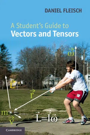 eBook - PDF
- Daniel A. Fleisch(Author)
- 2011(Publication Date)
- Cambridge University Press(Publisher)
6 Tensor applications This chapter provides examples of how to apply the tensor concepts contained in Chapters 4 and 5 , just as Chapter 3 provided examples of how to apply the vector concepts presented in Chapters 1 and 2 . As in Chapter 3 , the intent for this chapter is to include more detail about a small number of selected applications than can be included in the chapters in which tensor concepts are first presented. The examples in this chapter come from the fields of Mechanics, Elec-tromagnetics, and General Relativity. Of course, there’s no way to compre-hensively cover any significant portion of those fields in one chapter; these examples were chosen only to serve as representatives of the types of tensor application you’re likely to encounter in those fields. 6.1 The Inertia Tensor A very useful way to think of mass is this: mass is the characteristic of matter that resists acceleration. This means that it takes a force to change the velocity of any object with mass. You may find it helpful to think of moment of inertia as the rotational analog of mass. That is, moment of inertia is the characteristic of matter that resists angular acceleration, so it takes a torque to change the angular velocity of an object. Many students find that rotational motion is easier to understand by keeping the relationships between translational and rotational quantities in mind. So where translational motion dealt with position ( x ), velocity ( v ), and accelera-tion ( a ), rotational motion has the analogous quantities of angle ( θ ), angular velocity ( ω ), and angular acceleration ( α ). There are rotational analogs for many other quantities; the translational quantities of force ( F ), mass ( m ), and momentum ( p ) have the rotational equivalents of torque ( τ ), moment of inertia ( I ), and angular momentum ( L ). 159 No longer available |Learn more
- (Author)
- 2014(Publication Date)
- Library Press(Publisher)
The calculation considerably simplifies if we notice that by symmetry of the problem, the moments of inertia around all axes are equal: I x = I y = I z . Then where r 2 = x 2 + y 2 + z 2 is the distance from point r to the origin. This integral is easy to evaluate in the spherical coordinates, the volume element will be equal to d V = 4 πr 2 d r , where r goes from 0 to R . Thus, ________________________ WORLD TECHNOLOGIES ________________________ Moment of Inertia Tensor In three dimensions, if the axis of rotation is not given, we need to be able to generalize the scalar moment of inertia to a quantity that allows us to compute a moment of inertia about arbitrary axes. This quantity is known as the moment of Inertia Tensor and can be represented as a symmetric positive semi-definite matrix, I . This representation elegantly generalizes the scalar case: The angular momentum vector, is related to the rotation v elocity vector, ω by and the kinetic energy is given by as compared with in the scalar case. Like the scalar moment of inertia, the moment of Inertia Tensor may be calculated with respect to any point in space, but for practical purposes, the center of mass is almost always used. Definition For a rigid object of N point masses m k , the moment of Inertia Tensor has components given by , where ________________________ WORLD TECHNOLOGIES ________________________ and I 12 = I 21 , I 13 = I 31 , and I 23 = I 32 . (Thus I is a symmetric tensor.) Note that the scalars I ij with are called the products of inertia . Here I xx denotes the moment of inertia around the x -axis when the objects are rotated around the x-axis, I xy denotes the moment of inertia around the y -axis when the objects are rotated around the x -axis, and so on. These quantities can be generalized to an object with distributed mass, described by a mass density function, in a similar fashion to the scalar moment of inertia. eBook - PDF
- Nivaldo A. Lemos(Author)
- 2018(Publication Date)
- Cambridge University Press(Publisher)
4 Dynamics of Rigid Bodies The wheel is come full circle. William Shakespeare, King Lear, Act 5, Scene 3 Now that we are in possession of the necessary kinematic apparatus, we can proceed to examining some simple but important problems in the dynamics of rigid bodies, which requires us to take into account the causes of the motion: forces and torques. We start by considering two physical quantities which are essential in the study of the motion of a rigid body, the angular momentum and the kinetic energy. 4.1 Angular Momentum and Inertia Tensor The equations of motion for a rigid body can be written in the form dP dt = F , (4.1) dL dt = N , (4.2) where F is the total force and N is the total torque, P and L being the total linear momentum and total angular momentum, respectively. As discussed in Section 1.1, equations (4.1) and (4.2) are true only if the time rates of change are relative to an inertial reference frame and if certain restrictions are obeyed by the point with respect to which torque and angular momentum are calculated. In particular, (4.2) holds if the reference point for the calculation of N and L is at rest in an inertial reference frame – this is convenient if the rigid body is constrained to rotate about a fixed point – or is the centre of mass of the body. Let O be a fixed point or the centre of mass of a rigid body. From the point of view of the inertial frame depicted in Fig. 4.1, the total angular momentum of the body with respect to point O is L = N k=1 r k × p k = N k=1 m k r k × v k , (4.3) where N is the number of particles in the body and v k = (dr k /dt) is the velocity of the kth particle relative to point O as seen from the inertial frame . But r k is a constant vector in a Cartesian system attached to the body and we have 112 113 Angular Momentum and Inertia Tensor . . r k m k O S Fig. 4.1 O is a point of the body which remains fixed relative to the inertial frame or is the centre of mass of the body. eBook - PDF
- Jerry B. Marion(Author)
- 2013(Publication Date)
- Academic Press(Publisher)
We have therefore demonstrated two general procedures that may be used to diagonalize the Inertia Tensor. As was previously pointed out, these methods are not limited to the Inertia Tensor but are generally valid. Either procedure can, of course, be very complicated. For example, if we wish to use the rotation procedure in the most general case, we must first construct a matrix which describes an arbitrary rotation; this will entail three separate rotations, one about each of the coordinate axes. This 388 13 · DYNAMICS OF RIGID BODIES rotation matrix must then be applied to the tensor in a similarity trans-formation. The off-diagonal elements of the resulting matrix* must then be examined and values of the rotation angles determined so that these off-diagonal elements vanish. The actual use of such a procedure can tax the limits of human patience; however, in some simple situations this method of diagonalization can be used with profit. This is particularly true if the geometry of the problem indicates that only a simple rotation about one of the coordinate axes is necessary ; the rotation angle can then be evaluated without difficulty (see, for example, Problems 13-15, 13-17, and 13-18). The example of the cube illustrates the important point that the elements of the Inertia Tensor, the values of the principal moments of inertia, and the orientation of the principal axes for a rigid body all depend upon the choice of origin for the system. We recall, however, that in order for the kinetic energy to be separable into translational and rotational portions, the origin of the body coordinate system must, in general, be taken to coincide with the center of mass of the body. On the other hand, for any choice of the origin for any body there always exists an orientation of the axes which diagonalizes the Inertia Tensor and hence these axes become principal axes for that particular origin. Next, we seek to prove that the principal axes actually form an ortho-gonal set. eBook - PDF
- Richard Fitzpatrick(Author)
- 2012(Publication Date)
- Cambridge University Press(Publisher)
(7.3) Here, L = ∑ i=1,N m i r i × dr i /dt is the total angular momentum of the body (about the origin), and τ = ∑ i=1,N r i × F i is the total external torque (about the origin). The 105 106 Rigid body rotation ω r i O Fig. 7.1 A rigid rotating body. preceding equation is valid only if the internal forces are central in nature. However, this is not a particularly onerous constraint. Equation (7.3) describes how the angular momentum of a rigid body evolves in time under the action of the external torques. In the following, we shall consider only the rotational motion of rigid bodies, as their translational motion is similar to that of point particles [see Equation (7.2)] and, therefore, is fairly straightforward in nature. 7.3 Moment of Inertia Tensor Consider a rigid body rotating with fixed angular velocity ω about an axis that passes through the origin. (See Figure 7.1.) Let r i be the position vector of the ith mass element, whose mass is m i . We expect this position vector to precess about the axis of rotation (which is parallel to ω) with angular velocity ω. It, therefore, follows from Section A.7 that dr i dt = ω × r i . (7.4) Thus, Equation (7.4) specifies the velocity, v i = dr i /dt, of each mass element as the body rotates with fixed angular velocity ω about an axis passing through the origin. The total angular momentum of the body (about the origin) is written L = i=1,N m i r i × dr i dt = i=1,N m i r i × (ω × r i ) = i=1,N m i r 2 i ω − (r i · ω) r i , (7.5) where use has been made of Equation (7.4) and some standard vector identities. (See Section A.4.) The preceding formula can be written as a matrix equation of the form ⎛ ⎜ ⎜ ⎜ ⎜ ⎜ ⎜ ⎜ ⎜ ⎜ ⎝ L x L y L z ⎞ ⎟ ⎟ ⎟ ⎟ ⎟ ⎟ ⎟ ⎟ ⎟ ⎠ = ⎛ ⎜ ⎜ ⎜ ⎜ ⎜ ⎜ ⎜ ⎜ ⎜ ⎝ I xx I xy I xz I yx I yy I yz I zx I zy I zz ⎞ ⎟ ⎟ ⎟ ⎟ ⎟ ⎟ ⎟ ⎟ ⎟ ⎠ ⎛ ⎜ ⎜ ⎜ ⎜ ⎜ ⎜ ⎜ ⎜ ⎜ ⎝ ω x ω y ω z ⎞ ⎟ ⎟ ⎟ ⎟ ⎟ ⎟ ⎟ ⎟ ⎟ ⎠ , (7.6) eBook - PDF
- P. C. Deshmukh(Author)
- 2019(Publication Date)
- Cambridge University Press(Publisher)
The diagonal elements given by Eqs. 7.15a, d, and are summations of squares, and are thus always positive. The off-diagonal elements (product of inertia), can be either positive or negative, or even zero. Their values, as we can see from the nature of the integrands in Eq. 7.15, depend on the mass distributions about a specific point, and referenced to a particular orientation of the coordinate axes. The Inertia Tensor therefore contains information about how the mass of the object is distributed about its center of mass and with respect to a particular orientation of the coordinate system. The matrix multiplication in Eq. 7.17 elegantly reveals in a compact form that the angular momentum of a rigid body is not necessarily parallel to the angular velocity. The elements of the Inertia Tensor provide a measure of the components of the spin angular momentum in terms of the mass distribution of the spinning body, and the components of the angular velocity. The Inertia Tensor thus enables us write the relation between the spin angular momentum and the spin angular velocity in a neat form. It also helps write the relationship between the spin angular speed and the rotational kinetic energy in a simple form. In Eq. 7.8f, and Eq. 7.9, the rotational kinetic energy was identified as T I rotational kinetic energy = ω 2 2 . It has a quadratic dependence on the angular speed. The moment of inertia is, however, a tensor, given by Eq. 7.18. Retaining the same form, the rotational kinetic energy is therefore written in terms of the Inertia Tensor, using matrix multiplication rules, as T I I I I I x y z xx xy xz yx yy rotational kinetic energy = − − − × 1 2 1 3 {[ ] } ω ω ω − − − × × I I I I yz zx zy zz x y z 3 3 3 1 ω ω ω = 1 2 ω ω † ] . (7.19) We can also get the same result by following the slightly lengthy procedure such as in Eq.
Index pages curate the most relevant extracts from our library of academic textbooks. They’ve been created using an in-house natural language model (NLM), each adding context and meaning to key research topics.