Multipole Expansion

5 Key excerpts on "Multipole Expansion"

• 

  eBook - ePub

  The Electromagnetic Field

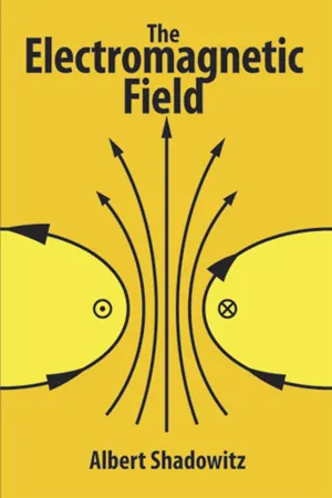
  • Albert Shadowitz(Author)
  • 2012(Publication Date)
  • Dover Publications

    (Publisher)

  The coefficient of the dipole term is a function of a vector, which is a more complicated quantity than a scalar. Similarly, the coefficient of the quadrupole term is a function of a quantity that is more complicated than a vector. In tensor analysis it is shown that this is a tensor of rank two. A vector is a tensor of rank one, a scalar is a tensor of rank zero. The word tensor has been used once before in this text in a purely formal way, in connection with the Maxwell stress tensor; its definition will be deferred until Chap. 14. The Multipole Expansion of the potential, which has been carried out to three terms above, applies to an arbitrary charge distribution. In particular, it is applicable to the distribution of charge which resides on any material body. When the body is a dielectric, i.e., one which is a nonconductor rather than a conductor or a semiconductor, then the first term in the Multipole Expansion generally vanishes, since the total charge on the body is zero unless special pains are taken to produce and maintain a net nonvanishing charge on it. The second term is also zero for most dielectrics in their normal state, i.e., when the bodies are not placed in an electric field. Most dielectrics do not possess a permanent dipole moment of their own. When a dielectric is placed in an electric field, however, the atoms of the dielectric are distorted and develop an electric dipole moment. The dielectric, itself, is said to acquire an induced dipole moment. A similar statement is also true, in general, for the third term of the Multipole Expansion. The quadrupole term, however, has an effect which drops off with distance much more quickly than does the dipole term; and this applies with even more force to higher-ordered terms. Consequently, for the study of dielectric materials in electric fields the electric dipole acquires a predominant importance, while the quadrupole and higher moments play a trivial role. Examples 1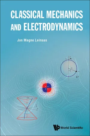

  Sign up to read

  Learn more about book
• 

  eBook - ePub

  Classical Mechanics and Electrodynamics

  • Jon Magne Leinaas(Author)
  • 2018(Publication Date)
  • WSPC

    (Publisher)

  r is sufficiently far away and the origin is chosen sufficiently close to the (center of the) charge distribution.

  The second term of the expansion is the electric dipole term,

  where we have introduced the electric dipole moment,

  This term gives a correction to the monopole term, and we note that for large r it falls off with distance like 1/r2 , while the monopole term falls off like 1/r. As a consequence, the monopole term will always dominate the dipole term for sufficiently large r (unless q = 0).

  We include one more term of the expansion in our discussion. This is the electric quadrupole term,

  with n = r/r as the unit vector in direct of the point r and Q

  n

  as the quadrupole moment about the axis n. It can be written as Q

  n

  = with

  as the quadrupole moment tensor.

  The electric field can now be expanded in the same way,

  with for the n′th term in the expansion. We give the explicit expressions for the first two terms. The monopole term is

  which is the Coulomb field of a point charge q located in the origin. The next term is

  with n = r/r as before. This field is called the electric dipole field.

  It should be clear from the above construction that the higher the multipole index n is, the faster the corresponding potential and electric field fall off with distance. Thus, for large r the n’th multipole term of the potential falls off like r

  –(n+1)

  , while the corresponding term in the expansion of the electric field field falls off like r

  –(n+2)

  . When considering the electric field far from the charges, it is often sufficient to consider only the first terms of the Multipole Expansion. In particular that is the case when we are interested in electromagnetic radiation far from the source, as we shall soon consider. In that case the field is determined by the time derivatives of the multipole moments. Since the total charge is conserved there will be no contribution from the monopole term, but for large r

  Sign up to read

  Learn more about book
• 

  eBook - PDF

  Introduction to Continuous Symmetries

  From Space-Time to Quantum Mechanics

  • Franck Laloë, Nicole Ostrowsky, Daniel Ostrowsky(Authors)
  • 2023(Publication Date)
  • Wiley-VCH

    (Publisher)

  A slightly different problem can also be treated, the interaction of the charges of S with an electric potential created by other charges (all outside S ). The result also involves the Q m l . In quantum mechanics, the Q m l become irreducible tensor operators T (K=l) Q=m . The Wigner–Eckart theorem can be applied to them. We shall continue the discussion in § 2, considering a system of stationary currents instead of motionless charges. This will lead to the introduction of “magnetic multipole moments” M m l , whose properties are fairly similar to those of the Q m l , except that they have opposite parity. § 3 will provide some examples of this formalism: electric quadrupole of atomic or nuclear levels, selection rules for multipole transitions between different levels. 415 COMPLEMENT C VIII • Comment: We will remain within the framework of electrostatics or magnetostatics (density of charges ρ and currents j varying very slowly in time). This restriction is not essential: one can reason in a more general way, within the framework of Maxwell’s equations taking into account the effects of radiation propagation. This leads to more elaborate computations, and it is useful to introduce the concept of “vector” spherical harmonics (analog to the “scalar” harmonics Y m l ), which are the eigenfunctions common to J 2 and J z for a vector field (instead of a scalar function, which has only one component). The interested reader may consult chapter 16 of [46], or the Collège de France teaching course of C. Cohen-Tannoudji (1973–1974), available online. 1. Electric multipole moments 1-a. Expanding the potential outside a system of charges Consider a density of charges ρ(r), localized in a volume V 0 , and note S 0 a sphere of radius R 0 , centered at the origin, containing V 0 (figure 1): ρ(r) = 0 if r > R 0 (1) We wish to calculate the potential V and the electric field E created by this system of charges outside the sphere S 0 .

  Sign up to read

  Learn more about book
• 

  eBook - PDF

  Generalized Calculus with Applications to Matter and Forces

  • Luis Manuel Braga de Costa Campos(Author)
  • 2014(Publication Date)
  • CRC Press

    (Publisher)

  A quadrupole is (Section 8.3) the limit of opposite dipoles and involves second-order derivatives of the unit impulse; since it has two axes, it is no longer generally axisymmetric, and the quadrupole moment is represented by a matrix. A three-dimensional charge distribution, like its two-dimensional counterpart, can be decomposed into a superposition of multipolar fields, with an important difference: (1) the two-dimensional multipoles have moments that are complex numbers; (2) the three-dimensional multipoles have moments of increasing complexity, namely, a scalar, a vector, a matrix, and a tensor, respectively, for mono-, di-, quadru-, and multipoles. The differences between the electrostatic (magnetostatic) field in space are greater than in the plane [Chapter I.24 (Chapter I.26)]: (1) the electrostatic field is irrotational, and is always represented by a scalar potential in two (Section I.24.2), three (Sections 8.1 through 8.3), or higher (Sections 9.7 through 9.9) dimensions; (2) the magnetostatic field is sole-noidal and is represented by a pseudoscalar field function in two dimensions (Section I.26.2) and by a vector potential (Section 8.4) in three dimensions; and (3) the three-dimensional vector potential reduces to a scalar stream function not only in the plane case but also in the three-dimensional axisymmetric case (Sections 6.2 through 6.7). Both the electrostatic (magnetostatic) fields have a multipolar expansion for the scalar (vector) potential [Section 8.3 (Section 8.4)]. The lowest-order term in the vector multipolar expansion for the magnetostatic potential corresponds to a point current; it is specified by a unit impulse like the electrostatic monopole, but has a vector direction 562 Generalized Calculus with Applications to Matter and Forces and is axisymmetric, corresponding to a magnetic dipole (Section 8.5).

  Sign up to read

  Learn more about book
• 

  eBook - PDF

  A Condensed Course of Quantum Mechanics

  • Pavel Cejnar(Author)
  • 2021(Publication Date)
  • Karolinum Press, Charles University

    (Publisher)

  157 One has: e i ~ k · ~x = 4 π ∞ ∑ l =0 + l ∑ m = -l i l j l ( kr ) Y * lm ~ k k Y lm ( ~x x ) (cf. Sec. 6.3) To include the polarization, we introduce circular & linear polarization bases in a general coordinate system: n ~e ± = ∓ 1 √ 2 ( ~n x ± i~n y ) ~e 0 = ~n z Arbitrary lin. polarization vector ~ ε ≡ ( ε x ~n x + ε y ~n y + ε z ~n z ) = q 4 π 3 ∑ ν =0 , ± 1 Y * 1 ν ( ~ ε ) ~e ν Note: the circular polarization vector ~e 0 is present because the evaluation is done in a general system unrelated to ~ k . Introduce a “vector spherical function” with total angular momentum (multi-polarity) λ : ~ Y lλμ ( ~x x ) = ∑ ν,m C λμ 1 νlm ~e ν Y lm ( ~x x ) ⇔ ~e ν Y lm ( ~x x ) = ∑ λ,μ C λμ 1 νlm ~ Y lλμ ( ~x x ) ~ ε e i ~ k · ~x = (4 π ) 3 2 3 X λ,μ X l,m X ν i l C λμ 1 νlm Y * 1 ν ( ~ ε ) Y * lm ~ k k j l ( kr ) ~ Y lλμ ( ~x x ) | {z } spatial dependence For each multipolarity λ it is possible to separate terms with both parities: electric (E) & magnetic (M) components. From the resulting expansion one can construct transition probabilities for E λ & M λ transitions. The above dipole approximation is identified as E1. J Historical remark 1900’s-10’s: Multipole Expansion of elmg. field elaborated within the classical theory 1940’s-50’s: Multipole Expansion applied in QM (M.E. Rose et al. ) 6. SCATTERING THEORY Description of the processes induced by scattering of particles belongs to the most important application domains of quantum theory. Knowing the interaction Hamil-tonian between the particles and the initial state, can one predict all outcomes & probabilities? And inversely: knowing the initial & final states, can one determine the interaction? This may resemble a task to analyze an internal structure of a watch by detecting tiny parts shot out when the thing is smashed on an anvil. In the quantum world, this is often the only research method available. The scattering theory is a rather wide area, of which we are going to taste only a little bit.

  Sign up to read

  Learn more about book