Oscillations

10 Key excerpts on "Oscillations"

• 

  eBook - PDF

  A Concise Handbook of Mathematics, Physics, and Engineering Sciences

  • Andrei D. Polyanin, Alexei Chernoutsan(Authors)
  • 2010(Publication Date)
  • CRC Press

    (Publisher)

  Chapter P4 Oscillations and Waves P4.1. Oscillations ◮ General definitions. Oscillations are repetitive variations in the state of a system such that the state parameters vary in time according to a periodic or almost periodic law. If Oscillations occur without external action due to system deviation from a stable equilibrium, the Oscillations are said to be free or natural . If the Oscillations occur under the action of an external periodic force, then they are said to be forced . The Oscillations are characterized by their period T and frequency ν = 1 /T (measured in hertzs : 1 Hz = 1 s – 1 ). The term vibrations is often used in a narrower sense to mean mechanical Oscillations, but sometimes is used synonymously with Oscillations. P4.1.1. Harmonic Oscillations. Composition of Oscillations ◮ Simple harmonic Oscillations. An oscillation of a quantity x is said to be a simple harmonic oscillation (or simple harmonic motion ) if x varies in time t by the law x = A cos( ωt + ϕ 0 ), (P4. 1 . 1 . 1 ) where A is the amplitude , ϕ = ωt + ϕ 0 is the phase , ϕ 0 is the initial phase , and ω = 2 π/T is the angular or circular frequency of the oscillation. The first and second time-derivatives of the quantity x , ˙ x = – Aω sin( ωt + ϕ 0 ) = Aω cos ( ωt + ϕ 0 + π/ 2 ) , ¨ x = – Aω 2 cos( ωt + ϕ 0 ) = Aω 2 cos( ωt + ϕ 0 + π ), (P4. 1 . 1 . 2 ) oscillate harmonically with the same frequency but with amplitudes ωA and ω 2 A and with the phase shifts π/ 2 and π , respectively. Example. If the initial values (at t = 0 ) of the quantity x and its derivative, x ( 0 ) = x 0 and ˙ x ( 0 ) = v 0 , are known, then the amplitude and the initial phase of the oscillation can be determined. The equations x 0 = A cos ϕ 0 and v 0 = – ωA sin ϕ 0 allow one to find A = radicalbig x 2 0 + ( v 0 /ω ) 2 and tan ϕ 0 = – v 0 / ( ωx 0 ).

  Sign up to read

  Learn more about book
• 

  eBook - PDF

  Principles of Engineering Physics 1

  • Md Nazoor Khan, Simanchala Panigrahi(Authors)
  • 2017(Publication Date)
  • Cambridge University Press

    (Publisher)

  1 Oscillations and Waves 1.1 Introduction Objects subjected to restoring forces when displaced from their normal positions and released, perform to and from or vibrating motions. They move back and forth along a path, repeating over and over again, a series of motions. Such motion of constant frequency is called periodic motion or harmonic motion and objects performing such type of motion are called harmonic oscillators. In this book, it is tacitly assumed that there is a linear relationship between force and displacement; frequency remains constant throughout the motion. In real systems however, the linear behavior, implicit in simple harmonic motion, is rarely obeyed. If the frequency of the oscillatory system is not constant, then it is called anharmonic motion – its study is beyond the scope of this book due to its mathematical complexities. In oscillatory systems, it is not necessarily the bodies themselves who execute Oscillations; bodies may be at rest. If the physical properties of a system undergo changes in an oscillatory manner, the system will also be called an oscillatory system. The electromagnetic energy transfer between the capacitor and inductor in a tank circuit used in electronic gadgets, variation of pressure in air due to propagation of sound waves, vibration of the diaphragm of a speaker in sound systems, flow of alternating current, variation of electric and magnetic vectors during propagation of electromagnetic waves, etc., are examples of oscillatory systems. 1.1.1 Parameters of an oscillatory system i. Mean position The position of the oscillating body when there is no oscillation is called the mean position or equilibrium position. This is the rest position of the oscillating body. 2 Principles of Engineering Physics 1 ii. Amplitude ( r ) It is the absolute value of the maximum displacement of the oscillating particle from its mean position or equilibrium position.

  Sign up to read

  Learn more about book
• 

  eBook - PDF

  Wave Optics

  Basic Concepts and Contemporary Trends

  • Subhasish Dutta Gupta, Nirmalya Ghosh, Ayan Banerjee(Authors)
  • 2015(Publication Date)
  • CRC Press

    (Publisher)

  25 Oscillations and vibrations constitute one of the major areas of study in physics. Most systems can oscillate freely. Generally, heavier ones have low oscillation frequency while the lighter ones have large frequencies. The vari-ety of phenomena exhibiting repetitive motions have been discussed nicely by French [1]: “Systems can vibrate freely in a large variety of ways. Broadly speaking, the predominant natural vibrations of 1 2 Wave Optics: Basic Concepts and Contemporary Trends small objects are likely to be rapid, and those of large ob-jects are likely to be slow. A mosquito’s wings, for example, vibrate hundreds of times per second and produce an audible note. The whole earth, after being jolted by an earthquake, may continue to vibrate at the rate of about one oscilla-tion per hour. The human body itself is a treasure-house of vibratory phenomena.” All the above phenomena have one thing in common, i.e., repetitive motion or periodicity. The same pattern of displacement is repeated over and over again. It can be simple or complicated. Irrespective of the nature of Oscillations, the pattern is generally represented by plots where the horizontal axis represents the steady progress of time. Such pictures make it easy to recognize one cycle or one period of oscillation, which keeps on repeating. 1.1 Sinusoidal Oscillations Sinusoidal Oscillations take place in a vast majority of mechanical systems. This is due to the fact that in most cases, the restoring force is proportional to the displacement. Such motion is always possible if the displacement is small enough. In general the restoring force F can have the following dependence on the displacement x : F ( x ) = − ( k 1 x + k 2 x 2 + k 3 x 3 + ... ) . (1.1) For small displacements we can ignore the terms proportional to x 2 , x 3 and other higher-order terms. This leads to an equation of motion m d 2 x dt 2 = − k 1 x, (1.2) which has a solution of the form x = A sin( ωt + φ 0 ) , ω = radicalbigg k 1 m .

  Sign up to read

  Learn more about book
• 

  eBook - PDF

  Applied Structural and Mechanical Vibrations

  Theory and Methods, Second Edition

  • Paolo L. Gatti(Author)
  • 2014(Publication Date)
  • CRC Press

    (Publisher)

  In practical cases, it is often the ability to reproduce the data by a controlled experiment that pro-vides a general criterion to distinguish between the two. 1.3 SOME DEFINITIONS AND METHODS As stated in the introduction, the particular behaviour of a particle, a body or a complex system that moves about an equilibrium position is called oscil-latory motion. It is then natural to try a description of such a particle, body or system by an appropriate function of time x ( t ), whose physical meaning depends on the scope of the investigation and, as often happens in practice, on the available measuring instrumentation: it might be displacement, veloc-ity, acceleration, stress or strain in structural dynamics; pressure or density in acoustics; current or voltage in electronics or any other time-varying quantity. A function that repeats itself exactly after certain intervals of time is called periodic . The simplest case of periodic motion is called harmonic (or sinusoidal) and is mathematically represented by a sine or cosine function; for example x t X t ( 29 = -( 29 cos ω θ (1.4) where: X is the maximum , or peak amplitude (in the appropriate units) ω t − θ is the phase angle (in radians) ω is the angular frequency (in rad/s) θ is the initial phase angle (in radians), which, in turn, depends on the choice of the time origin and can be taken equal to zero if there is no rela-tive reference to other sinusoidal functions The time between two identical conditions of motion is the period T . It is measured in seconds and is the inverse of the frequency ν = ω /2 π , which is expressed in hertz (Hz, with dimensions of s −1 ). As is probably well known to the reader, frequency represents the number of cycles per unit time and for the harmonic function (Equation 1.4) we have the relations ω πν π ω = = = 2 1 2 , T ν (1.5) A plot of Equation 1.4, amplitude versus time, is illustrated in Figure 1.1 where the peak amplitude is taken as X = 1 and the initial phase angle is θ = 0.

  Sign up to read

  Learn more about book
• 

  eBook - PDF

  Mechanical Science for Technicians

  Volume 2

  • Ian McDonagh(Author)
  • 2014(Publication Date)
  • Arnold

    (Publisher)

  9 Oscillations 9.1 Periodic time and frequency An oscillation is defined as a to-and-fro motion about a mean position and is completed when the motion of M in fig. 9.1 is from 0 to A to B and back to 0. Mean position 0 t fc M m i Fig. 9.1 Definition of an oscillation The time required to complete one cycle of the motion is known as the period or periodic time, T, of the oscillation, and the number of cycles made per unit time is known as the frequency, /, of the oscillation. If the periodic time for each successive oscillation is the same (i.e. 7), then frequency = periodic time / -I T which it is useful to remember. The unit for frequency is the hertz (Hz), and for periodic time the second (s). It is important to note that 1 Hz = 1 cycle/second or 1 oscillation/second or 1 revolution/second 9.2 Displacement and amplitude In oscillatory motion, the displacement, x, is measured outwards from either side of the mean position, as shown in fig. 9.2. The maximum displacement on either side of the mean position is known as the amplitude of the motion. 180 or ^ ^ Mean position r _ — 1 Amplitude — I ί x 2 r 1 I Amplitude -~t-— —»-Fig. 9.2 Measurement of displacement and amplitude 9.3 Simple harmonic motion The most common form of oscillatory motion is simple harmonic motion (S.H.M.). An oscillating body will have S.H.M. if, at any instant during the cycle, i) the acceleration of the body is proportional to its displacement from the mean position, and ii) the acceleration of the body is always directed towards the mean position. Consider the motion of Q, which is the projection of P on to the line AB in fig. 9.3. P is rotating in a circle of radius r with uniform angular velocity , causing Q to oscillate between A and B about the mean position 0. In the position shown, where P has rotated through angle Θ in time t, i.e. 0 = , Fig. 9.3 Simple harmonic motion 181

  Sign up to read

  Learn more about book
• 

  eBook - PDF

  Physics for Scientists and Engineers with Modern Physics

  • Raymond Serway, John Jewett(Authors)
  • 2018(Publication Date)
  • Cengage Learning EMEA

    (Publisher)

  385 P A R T 2 Oscillations and Mechanical Waves Falling drops of water cause a water surface to oscillate. These Oscillations are associated with circular waves moving away from the point at which the drops fall. In Part 2 of the text, we will explore the principles related to Oscillations and waves. ( Ziga Camernik/Shutterstock) In Part 1 of this text, we focused on one particular energy transfer term in Equation 8.2: work W. In Parts 2 through 5, we will focus our efforts in each part on a new term in Equation 8.2. Here in Part 2, we will investigate the term T MW : transfer of energy by mechanical waves. We begin this new part of the text by studying a special type of motion called periodic motion, the repeating motion of an object in which it con- tinues to return to a given position after a fixed time interval. The repet- itive movements of such an object are called Oscillations. We will focus our attention on a special case of periodic motion called simple harmonic motion. All periodic motions can be modeled as combinations of simple harmonic motions. Simple harmonic motion also forms the basis for our understanding of mechanical waves. Sound waves, seismic waves, waves on stretched strings, and water waves are all produced by some source of oscillation. As a sound wave travels through the air, elements of the air oscillate back and forth; as a water wave travels across a pond, elements of the water oscillate up and down and backward and forward. To explain many other phenomena in nature, we must understand the concepts of Oscillations and waves. For instance, although skyscrap- ers and bridges appear to be rigid, they actually oscillate, something the architects and engineers who design and build them must take into account. To understand how radio and television work, we must under- stand the origin and nature of electromagnetic waves and how they prop- agate through space.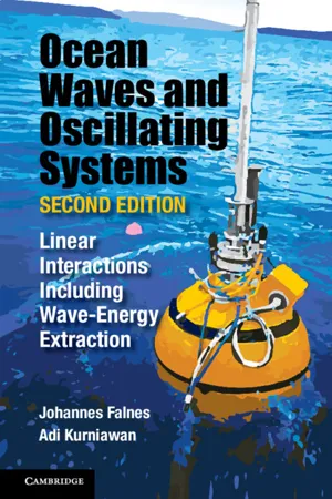

  Sign up to read

  Learn more about book
• 

  eBook - PDF

  Ocean Waves and Oscillating Systems: Volume 8

  Linear Interactions Including Wave-Energy Extraction

  • Johannes Falnes, Adi Kurniawan(Authors)
  • 2020(Publication Date)
  • Cambridge University Press

    (Publisher)

  CHAPTER TWO Mathematical Description of Oscillations In this chapter, which is a brief introduction to the theory of Oscillations, a simple mechanical oscillation system is used to introduce concepts such as free and forced Oscillations, state-space analysis and representation of sinusoidally varying physical quantities by their complex amplitudes. In order to be some- what more general, causal and noncausal linear systems are also looked at and Fourier transform is used to relate the system’s transfer function to its impulse response function. With an assumption of sinusoidal (or ‘harmonic’) Oscillations, some important relations are derived which involve power and stored energy on one hand and the parameters of the oscillating system on the other hand. The concepts of resonance and bandwidth are also introduced. 2.1 Free and Forced Oscillations of a Simple Oscillator Let us consider a simple mechanical oscillator in the form of a mass–spring– damper system. A mass m is suspended through a spring and a mechanical damper, as indicated in Figure 2.1. Because of the application of an external force F , the mass has a position displacement x from its equilibrium position. Newton’s law gives m ¨ x = F + F R + F S , (2.1) where F S is the spring force and F R is the damper force. If we assume that the spring and the damper have linear characteristics, then we can write F S = −Sx and F R = −R ˙ x, where the ‘stiffness’ S and the ‘mechanical resistance’ R are coefficients of proportionality, independent of the displace- ment x and the velocity u = ˙ x. Thus, we have the following linear differential equation with constant coefficients: m ¨ x + R ˙ x + Sx = F , (2.2) where an overdot is used to denote differentiation with respect to time t. 6 2.1 FREE AND FORCED Oscillations OF A SIMPLE OSCILLATOR 7 Figure 2.1: Mechanical oscillator in the form of a mass–spring–damper system.

  Sign up to read

  Learn more about book
• 

  eBook - PDF

  Foundations of Classical Mechanics

  • P. C. Deshmukh(Author)
  • 2019(Publication Date)
  • Cambridge University Press

    (Publisher)

  We have so far considered Oscillations of an object about a point of stable equilibrium. There is also an energy associated with the ‘disturbance’ that is oscillating. In a frictionless environment, this energy is conserved, changing at every instant between kinetic and potential forms. The mean (i.e., average over one period) kinetic energy and mean potential energy are respectively given by: 133 Small Oscillations and Wave Motion KE mq m t m = 1 2 2 4 2 0 0 2 2 0 2  = − + = [ sin( )] , ω λ ω φ λ ω (4.28a) PE q t = 1 2 2 4 2 0 2 2 κ κ λ ω φ κ λ = + = [ cos( )] , (4.28b) where we have used 1 2 2 2 ( ( ω ω dt dt = = . We note, however, that < PE > = < KE >, since ω κ 0 2 = m . (4.29) The total energy of the oscillating disturbance, however, remains localized in space in a tiny region of space about its mean position. 4.3 WAVE MOTION We shall now extend the idea of displacement of the oscillator about its mean position to a disturbance about the mean position. In order to develop a rather general analysis of the wave motion, we deliberately avoid the question about disturbance of just what, i.e., we talk about the disturbance without worrying about just what is being disturbed. Essentially, this will allows us a generalization of the vocabulary we have employed so far to accommodate electromagnetic fields. The oscillators we have talked about so far are essentially mechanical oscillators, like the mass attached to a spring, or a simple pendulum, executing small Oscillations. The Oscillations that we shall now talk about may be more generally referred to as a time-dependent disturbance, such as the amplitude of an electric and the magnetic vector of an electromagnetic wave. In what follows, the term disturbance would continue to include the displacement of a mechanical oscillator about its mean position, but will also include the amplitude of an electric and magnetic vector of an electromagnetic field.

  Sign up to read

  Learn more about book
• 

  eBook - PDF

  Simulations of Oscillatory Systems

  with Award-Winning Software, Physics of Oscillations

  • Eugene I. Butikov(Author)
  • 2015(Publication Date)
  • CRC Press

    (Publisher)

  We consider both steady-state sinusoidal forced Oscillations, which take place later than a sufficiently large time interval elapsed after the driving force started to operate, and transient processes, the latter depending on the initial conditions. The decomposition of a transient process onto the sum of sinusoidal Oscillations of a constant amplitude, which have the frequency of the external force, and damped free Oscillations with the natural frequency, are examined. 33 34 CHAPTER 3. FORCED Oscillations IN A LINEAR SYSTEM 3.1.1 Basic Concepts In the conventional classification of Oscillations by their mode of excitation, oscil-lations are called forced if an oscillator is subjected to an external periodic influ-ence whose effect on the system can be expressed by a separate term, a periodic function of the time, in the differential equation of motion. We are interested in the response of the system to the periodic external force. The behavior of oscillatory systems under periodic external forces is one of the most important topics in the theory of Oscillations. A noteworthy distinctive char-acteristic of forced Oscillations is the phenomenon of resonance, in which a small periodic disturbing force can produce an extraordinarily large response in the os-cillator. Resonance is found everywhere in physics and so a basic understanding of this fundamental problem has wide and various applications. The phenomenon of resonance depends upon the whole functional form of the driving force and occurs over an extended interval of time rather than at some particular instant. In the case of unforced (free, or natural) Oscillations of an isolated system, motion is initiated by an external influence acting before a particular instant. This influence determines the mechanical state of the system, that is, the displacement and the velocity of the oscillator, at the initial instant. These in turn determine the amplitude and phase of subsequent free Oscillations.

  Sign up to read

  Learn more about book
• 

  eBook - ePub

  Experiments and Demonstrations in Physics

  Bar-Ilan Physics Laboratory

  • Yaakov Kraftmakher(Author)
  • 2014(Publication Date)
  • WSPC

    (Publisher)

  et al (2002) observed Oscillations of a pendulum with one of three damping effects: friction not depending on the velocity (sliding friction), linear dependence on the velocity (eddy currents in a metal plate), and quadratic dependence on the velocity (air friction).

  For other experiments with pendulums, see Lapidus (1970); Schery (1976); Hall and Shea (1977); Simon and Riesz (1979); Hall (1981); Yurke (1984); Eckstein and Fekete (1991); Ochoa and Kolp (1997); Peters (1999); Lewowski and Woźniak (2002); LoPresto and Holody (2003); Parwani (2004); Coullet et al (2005); Ng and Ang (2005); Jai and Boisgard (2007); Gintautas and Hübler (2009); Mungan and Lipscombe (2013).

  Theoretical background. For a mathematical pendulum with friction, the motion equation is

  where m is the mass, a is the acceleration, x is the displacement, v is the velocity, k and λ are coefficients of proportionality, x′ = v = dx/dt, and x″ = d2 x/dt2 . The solution to this equation describing free Oscillations is

  where A and φ1 depend on the initial conditions. The natural frequency of the system is ω0 = (k/m)½ = (g/l)½ , the decay of free Oscillations is governed by the decay constant δ = λ/2m, and the angular frequency Ω is somewhat lower than ω0 : Ω2 = ω0 2 – δ2 .

  The transient process after application of a periodic driving force deserves special consideration. Whenever forced Oscillations start, a process occurs leading to steady Oscillations. This transient process is caused by the superposition of forced and free Oscillations. Landau and Lifshitz (1982) and Pippard (1989) considered the problem in detail, and this analysis is partly reproduced here. For a driven mathematical pendulum

  Sign up to read

  Learn more about book