Speculation, Trading, and Bubbles

José Scheinkman, Kenneth Arrow, Patrick Bolton, Joseph E. Stiglitz, Sanford Grossman

• Editore: Columbia University Press
• Anno: 2014
• ISBN:
  9780231537636
• Argomento: Business
• Categoria: Business generale

As long as there have been financial markets, there have been bubbles—those moments in which asset prices inflate far beyond their intrinsic value, often with ruinous results. Yet economists are slow to agree on the underlying forces behind these events. In this book José A. Scheinkman offers new insight into the mystery of bubbles. Noting some general characteristics of bubbles—such as the rise in trading volume and the coincidence between increases in supply and bubble implosions—Scheinkman offers a model, based on differences in beliefs among investors, that explains these observations.

Other top economists also offer their own thoughts on the issue: Sanford J. Grossman and Patrick Bolton expand on Scheinkman's discussion by looking at factors that contribute to bubbles—such as excessive leverage, overconfidence, mania, and panic in speculative markets—and Kenneth J. Arrow and Joseph E. Stiglitz contextualize Scheinkman's findings.

APPENDIX: A FORMAL MODEL

A.1 THE BASIC MODEL

I first exposit a simple model to illustrate the role of costly shorting and differences in beliefs in generating bubbles and the association between bubbles and trading. Consider four periods t = 1, 2, 3, 4; a single good; and a single risky asset in finite supply S. In addition to the risky asset, there also exists a risk-free technology. An investment of δ ≤ 1 units of the good in the risk-free technology at t yields one unit in period t + 1. Assume there are a large number of risk-neutral investors that only value consumption in the final period t = 4. Each investor is endowed with an amount W₀ of the good.

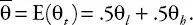
The risky asset produces dividends at times t = 2, 3, 4. At each t = 2, 3, 4 each unit of the risky asset pays a dividend θ_t Є {θ_l, θ_h} with θ_h > θ_l. In what follows, I will refer to θ_h (θ_l) as the high (resp. low) dividend. Dividends at any t are independent of past and future dividends.¹ The probability that θ_t = θ_l is .5, and we write

Assets are traded at t = 1, 2, 3, 4. If a dividend is paid in period t, trading occurs after the dividend is distributed—that is, the asset trades ex-dividend and the buyer of the asset in period t has the rights to all dividends from time t + 1 on. Thus in the final period t = 4, the price of the asset p₄ = 0, since there are no dividends paid after period 4. The price at time t = 1, 2, 3 depends on the expectations of investors regarding the dividends to be paid in the future. We first calculate the willingness to pay of a “rational” risk-neutral investor that is not allowed to resell the asset after she buys it. Since the investor is risk-neutral, at time t = 3 she is willing to pay

for a unit of the asset. In the absence of resale opportunities, at t = 2, the rational investor is willing to pay

. Finally, at t = 1 that same rational investor with no resale opportunities would be willing to pay

In addition, we suppose that at each t = 1, 2, 3, a signal s_t is observed after the dividend at t (if t > 1) is observed but before trading occurs at t. Each signal s_t assumes one of three values {0, 1, 2}, is independent of past realizations of the signal and of the dividends, and has no predictive power for future dividends. Thus the signal s_t is pure noise. There are, however, two sets of investors, A and B. Each set has many investors. Agents in group A are rational and understand that the distribution of future dividends is independent of s_t. Agents in B actually believe that s_t predicts θ_t+1 and that the probability that θ_t+1 = θ_h given s_t is:

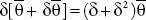
Thus agents in group B believe that the probability of a high dividend at t +1 increases with the observed s_t and that when s_t = 0(s_t = 2), θ_t+1 = θ_l(resp. θ_t+1 = θ_h) is more probable. All agents agree that s_t does not help predict θ_t+j for j≥2, and thus the only disagreement among investors is whether s_t can predict θ_t+1. To make agents in set B correct on average, and thus assure that ex-ante there are no optimistic or pessimistic investors, assume that the probability that s_t = 0 equals the probability that s_t = 2. Write q.<5 for this common probability, and observe that the probability that s_t = 1 is 1 − 2q>0.

In the case of binary random variables, forecasts have minimal precision² when the probability of each realization is 1/2. This is exactly the forecast of rational agents here. Agents in group B, after observing s_t = 1, also have the same minimal forecast precision. However, if they observe s_t = 0 or s_t = 2 they employ forecasts that have higher precision, since they (mistakenly) believe that one of the two possible events has a probability of 3/4. In this sense agents in group B have an exaggerated view of the precision of their beliefs.

At time t = 3, rational agents in group A are wil...