![]()
Chapter 1
Introduction
1.1 Introduction
Studies in the social sciences comparing two or more groups very often measure their participants on several criterion variables. The following are some examples:
- A researcher is comparing two methods of teaching second-grade reading. On a posttest the researcher measures the participants on the following basic elements related to reading: syllabication, blending, sound discrimination, reading rate, and comprehension.
- A social psychologist is testing the relative efficacy of three treatments on self-concept, and measures participants on academic, emotional, and social aspects of self-concept. Two different approaches to stress management are being compared.
- The investigator employs a couple of paper-and-pencil measures of anxiety (say, the State-Trait Scale and the Subjective Stress Scale) and some physiological measures.
- A researcher comparing two types of counseling (Rogerian and Adlerian) on client satisfaction and client self-acceptance.
A major part of this book involves the statistical analysis of several groups on a set of criterion measures simultaneously, that is, multivariate analysis of variance, the multivariate referring to the multiple dependent variables.
Cronbach and Snow (1977), writing on aptitude–treatment interaction research, echoed the need for multiple criterion measures:
Learning is multivariate, however. Within any one task a person’s performance at a point in time can be represented by a set of scores describing aspects of the performance…even in laboratory research on rote learning, performance can be assessed by multiple indices: errors, latencies and resistance to extinction, for example. These are only moderately correlated, and do not necessarily develop at the same rate. In the paired associate’s task, sub skills have to be acquired: discriminating among and becoming familiar with the stimulus terms, being able to produce the response terms, and tying response to stimulus. If these attainments were separately measured, each would generate a learning curve, and there is no reason to think that the curves would echo each other. (p. 116)
There are three good reasons that the use of multiple criterion measures in a study comparing treatments (such as teaching methods, counseling methods, types of reinforcement, diets, etc.) is very sensible:
- Any worthwhile treatment will affect the participants in more than one way. Hence, the problem for the investigator is to determine in which specific ways the participants will be affected, and then find sensitive measurement techniques for those variables.
- Through the use of multiple criterion measures we can obtain a more complete and detailed description of the phenomenon under investigation, whether it is teacher method effectiveness, counselor effectiveness, diet effectiveness, stress management technique effectiveness, and so on.
- Treatments can be expensive to implement, while the cost of obtaining data on several dependent variables is relatively small and maximizes information gain.
Because we define a multivariate study as one with several dependent variables, multiple regression (where there is only one dependent variable) and principal components analysis would not be considered multivariate techniques. However, our distinction is more semantic than substantive. Therefore, because regression and component analysis are so important and frequently used in social science research, we include them in this text.
We have four major objectives for the remainder of this chapter:
- To review some basic concepts (e.g., type I error and power) and some issues associated with univariate analysis that are equally important in multivariate analysis.
- To discuss the importance of identifying outliers, that is, points that split off from the rest of the data, and deciding what to do about them. We give some examples to show the considerable impact outliers can have on the results in univariate analysis.
- To discuss the issue of missing data and describe some recommended missing data treatments.
- To give research examples of some of the multivariate analyses to be covered later in the text and to indicate how these analyses involve generalizations of what the student has previously learned.
- To briefly introduce the Statistical Analysis System (SAS) and the IBM Statistical Package for the Social Sciences (SPSS), whose outputs are discussed throughout the text.
1.2 Type I Error, Type II Error, and Power
Suppose we have randomly assigned 15 participants to a treatment group and another 15 participants to a control group, and we are comparing them on a single measure of task performance (a univariate study, because there is a single dependent variable). You may recall that the t test for independent samples is appropriate here. We wish to determine whether the difference in the sample means is large enough, given sampling error, to suggest that the underlying population means are different. Because the sample means estimate the population means, they will generally be in error (i.e., they will not hit the population values right “on the nose”), and this is called sampling error. We wish to test the null hypothesis (H0) that the population means are equal:
H0 : μ1 = μ2
It is called the null hypothesis because saying the population means are equal is equivalent to saying that the difference in the means is 0, that is, μ1 − μ2 = 0, or that the difference is null.
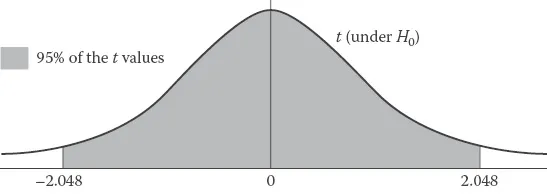
Now, statisticians have determined that, given the assumptions of the procedure are satisfied, if we had populations with equal means and drew samples of size 15 repeatedly and computed a t statistic each time, then 95% of the time we would obtain t values in the range −2.048 to 2.048. The so-called sampling distribution of t under H0 would look like this:
This sampling distribution is extremely important, for it gives us a frame of reference for judging what is a large value of t. Thus, if our t value was 2.56, it would be very plausible to reject the H0, since obtaining such a large t value is very unlikely when H0 is true. Note, however, that if we do so there is a chance we have made an error, because it is possible (although very improbable) to obtain such a large value for t, even when the population means are equal. In practice, one must decide how much of a risk of making this type of error (called a type I error) one wishes to take. Of course, one would want that risk to be small, and many have decided a 5% risk is small. This is formalized in hypothesis testing by saying that we set our level of significance (α) at the .05 level. That is, we are willing to take a 5% chance of making a type I error. In other words, type I error (level of significance) is the probability of rejecting the null hypothesis when it is true.
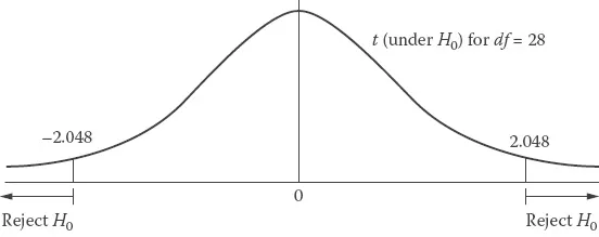
Recall that the formula for degrees of freedom for the t test is (n1 + n2 − 2); hence, for this problem df = 28. If we had set α = .05, then reference to Appendix A.2 of this book shows that the critical values are −2.048 and 2.048. They are called critical values because they are critical to the decision we will make on H0. These critical values define critical regions in the sampling distribution. If the value of t falls in the critical region we reject H0; otherwise we fail to reject:
Type I error is equivalent to saying the groups differ when in fact they do not. The α level set by the investigator is a subjective decision, but is usually set at .05 or .01 by most researchers. There are situations, however, when it makes sense to use α levels other than .05 or .01. For example, if making a type I error will not have serious substantive consequences, or if sample size is small, setting α = .10 or .15 is quite reasonable. Why this is reasonable for small sample size will be made clear shortly. On the other hand, suppose we are in a medical situation where the null hypothesis is equivalent to saying a drug is unsafe, and the alternative is that the drug is safe. Here, making a type I error could be quite serious, for we would be declaring the drug safe when it is not safe. This could cause some people to be permanently damaged or perhaps even killed. In this case it would make sense to use a very small α, perhaps .001.
Another type of error that can be made in conducting a statistical test is called a type II error. The type II error rate, denoted by β, is the probability of accepting H0 when it is false. Thus, a type II error, in this case, is saying the groups don’t differ when they do. Now, not only can either type of error occur, but in addition, they are inversely related (when other factors, e.g., sample size and effect size, affecting these probabilities are held constant). Thus, holding these factors constant, as we control on type I error, type II error increases. This is illustrated here for a two-group problem with 30 participants per group where the population effect size d (defined later) is .5:
α | β | 1 − β |
.10 | .37 | .63 |
.05 | .52 | .48 |
.01 | .78 | .22 |
Notice that, with sample and effect size held constant, as we exert more stringent control over α (from .10 to .01), the type II error rate increases fairly sharply (from .37 to .78). Therefore, the problem for the experimental planner is achieving an appropriate balance between the two types of errors. While we do not intend to minimize the seriousness of making a type I error, we hope to convince you throughout the course of this text that more attention should be paid to type II error. Now, the quantity in the last column of the preceding table (1 − β) is the power of a statistical test, which is the probability of rejecting the null hypothesis when it is false. Thus, power is the probability of making a correct decision, or of saying the groups differ when in fact they do. Notice from the table that as the α level decreases, power also decreases (given that effect and sample size are held constant). The diagram in Figure 1.1 should help to make clear why this happens.
The power of a statistical test is dependent on three factors:
- The α level set by the experimenter
- Sample size
- Effect size—How much of a difference the treatments make, or the extent to which the groups differ in the population on the dependent variable(s).
Figure 1.1 has already demonstrated that power is directly dependent on the α level. Power is h...