Data Analysis

A Model Comparison Approach To Regression, ANOVA, and Beyond, Third Edition

Charles M. Judd, Gary H. McClelland, Carey S. Ryan

• Publisher: Routledge
• Year: 2017
• Print ISBN: 9781138819825
• eBook ISBN: 9781317591207
• Topic: Psychology
• Subtopic: Education Theory & Practice
• Index: Psychology

Data Analysis: A Model Comparison Approach to Regression, ANOVA, and Beyond is an integrated treatment of data analysis for the social and behavioral sciences. It covers all of the statistical models normally used in such analyses, such as multiple regression and analysis of variance, but it does so in an integrated manner that relies on the comparison of models of data estimated under the rubric of the general linear model.

Data Analysis also describes how the model comparison approach and uniform framework can be applied to models that include product predictors (i.e., interactions and nonlinear effects) and to observations that are nonindependent. Indeed, the analysis of nonindependent observations is treated in some detail, including models of nonindependent data with continuously varying predictors as well as standard repeated measures analysis of variance. This approach also provides an integrated introduction to multilevel or hierarchical linear models and logistic regression. Finally, Data Analysis provides guidance for the treatment of outliers and other problematic aspects of data analysis. It is intended for advanced undergraduate and graduate level courses in data analysis and offers an integrated approach that is very accessible and easy to teach.

Highlights of the third edition include:

• a new chapter on logistic regression;
• expanded treatment of mixed models for data with multiple random factors;
• updated examples;

• an enhanced website with PowerPoint presentations and other tools that demonstrate the concepts in the book; exercises for each chapter that highlight research findings from the literature; data sets, R code, and SAS output for all analyses; additional examples and problem sets; and test questions.

1
Introduction to Data Analysis

This book is about data analysis. In the social and behavioral sciences we often collect batches of data that we hope will answer questions, test hypotheses, or disprove theories. To do so we must analyze our data. In this chapter, we present an overview of what data analysis means. This overview is intentionally abstract with few details so that the “big picture” will emerge. Data analysis is remarkably simple when viewed from this perspective, and understanding the big picture will make it much easier to comprehend the details that come later.

Overview of Data Analysis

The process of data analysis is represented by the following simple equation:

DATA = MODEL + ERROR

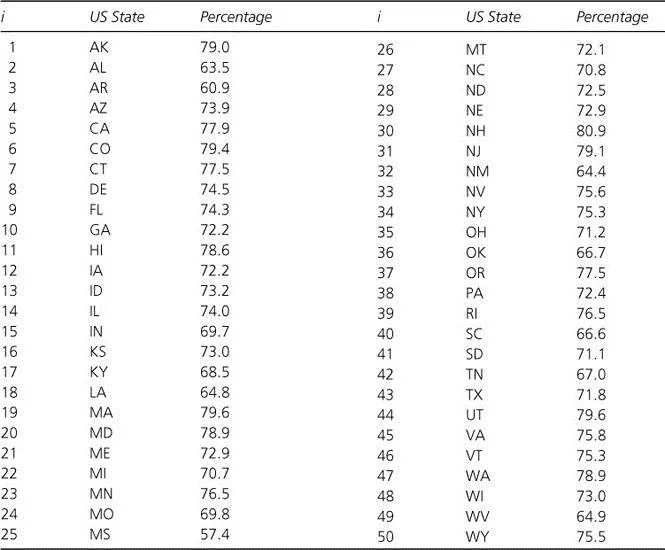
DATA represents the basic scores or observations, usually but not always numerical, that we want to analyze. MODEL is a more compact description or representation of the data. Our data are usually bulky and of a form that is hard to communicate to others. The compact description provided by the model is much easier to communicate, say, in a journal article, and is much easier to think about when trying to understand phenomena, to build theories, and to make predictions. To be a representation of the data, all the models we consider will make a specific prediction for each observation or element in DATA. Models range from the simple (making the same prediction for every observation in DATA) to the complex (making differential predictions conditional on other known attributes of each observation). To be less abstract, let us consider an example. Suppose our data were, for each state in the United States, the percentage of households that had internet access in the year 2013; these data are listed in Figure 1.1. A simple model would predict the same percentage for each state. A more complex model might adjust the prediction for each state according to the age, educational level, and income of the state’s population, as well as whether the population is primarily urban or rural. The amount by which we adjust the prediction for a particular attribute (e.g., educational level) is an unknown parameter that must be estimated from the data.

The last part of our basic equation is ERROR, which is simply the amount by which the model fails to represent the data accurately. It is an index of the degree to which the model mispredicts the data observations. We often refer to error as the residual—the part that is left over after we have used the model to predict or describe the data. In other words:

ERROR = DATA – MODEL

The goal of data analysis is then clear: We want to build the model to be a good representation of the data by making the error as small as possible. In the unlikely extreme case when ERROR = 0, DATA would be perfectly represented by MODEL.

Figure 1.1 Percentage of households that had internet access in the year 2013 by US state

How do we reduce the error and improve our models? One way is to improve the quality of the data so that the original observations contain less error. This involves better research designs, better data collection procedures, more reliable instruments, etc. We do not say much about such issues in this book, but instead leave those problems to texts and courses in experimental design and research methods. Those problems tend to be much more discipline specific than the general problems of data analysis and so are best left to the separate disciplines. Excellent sources that cover such issues are Campbell and Stanley (1963), Cook and Campbell (1979), Judd and Kenny (1981a), Maruyama and Ryan (2014), Reis and Judd (2014), Rosenthal and Rosnow (2008), and Shadish, Cook, and Campbell (2002). Although we often note some implications of data analysis procedures for the wise design of research, we in general assume that the data analyst is confronted with the problem of building the best model for data that have already been collected.

The method available to the data analyst for reducing error and improving models is straightforward and, in the abstract, the same across disciplines. Error can almost always be reduced (never increased) by making the model’s predictions conditional on additional information about each observation. This is equivalent to adding parameters to the model and using data to build the best estimates of those parameters. The meaning of “best estimate” is clear: we want to set the parameters of the model to whatever values will make the error the smallest. The estimation of parameters is sometimes referred to as “fitting” the model to the data. Our ideal data analyst has a limited variety of basic models. It is unlikely that any of these models will provide a good fit “off the rack”; instead, the basic model will need to be fitted or tailored to the particular size and bulges of a given data customer. In this chapter, we are purposely vague about how the error is actually measured and about how parameters are actually estimated to make the error as small as possible because that would get us into details to which we devote whole chapters later. But for now the process in the abstract ought to be clear: add parameters to the model and estimate those parameters so that the model will provide a good fit to the data by making the error as small as possible.

To be a bit less abstract, let us again consider the example of internet access by state. An extremely simple model would be to predict a priori (that is, without first examining the data) that in each state the percentage of households that has internet access is 75. This qualifies as a model according to our definition, because it makes a prediction for each of the 50 states. But in this model there are no parameters to be estimated from the data to provide a good fit by making the error as small as possible. No matter what the data, our model predicts 75. We will introduce some notation so that we have a standard way of talking about the particulars of DATA, MODEL, and ERROR. Let Y_i represent the ith observation in the data; in this example Y_i is simply the percentage of households that have internet access for the ith state. Then our basic equation:

DATA = MODEL + ERROR

for this extremely simple model becomes:

Y_i = 75 + ERROR

We can undoubtedly improve our model and reduce the error by using a model that is still simple but has one parameter: predict that the percentage is the same in all states, but leave the predicted value as an unspecified parameter to be estimated from the data. For example, the average of all 50 percentages might provide a suitable estimate. We will let β₀ represent the unknown value that is to be estimated so that our slightly more complex, but still simple, model becomes:

Y_i = β₀ + ERROR

It is important to realize that we can never know β₀ for certain; we can only estimate it.

We can make our model yet more complex and reduce the error further by adding more parameters to make conditional predictions. For example, innovations reputedly are adopted on the east and west coasts before the middle of the country. We could implement that in a model that starts with a basic percentage of internet use (β₀) for all states, which is adjusted upward by a certain amount (β₁) if the state is in the Eastern or Pacific time zones and reduced by that same amount if the state is in the Central or Mountain time zones. More formally, our basic equation now has a more complex representation, namely:

Y_i = β₀ + β₁ + ERROR if the state is in the Eastern or Pacific time zones

Y_i = β₀ – β₁ + ERROR if the state is in the Central or Mountain time zones

In other words, our model and its prediction would be conditional on the time zone in which the state is located.

Another slightly more complex model would make predictions conditional on a continuous, rather than a categorical, predictor. For example, we might make predictions conditional on the proportion of college graduates in a state, presuming that college gradua...

Table of contents

• Cover
• Title
• Copyright
• Contents
• Preface
• 1 Introduction to Data Analysis
• 2 Simple Models: Definitions of Error and Parameter Estimates
• 3 Simple Models: Models of Error and Sampling Distributions
• 4 Simple Models: Statistical Inferences about Parameter Values
• 5 Simple Regression: Estimating Models with a Single Continuous Predictor
• 6 Multiple Regression: Models with Multiple Continuous Predictors
• 7 Moderated and Nonlinear Regression Models
• 8 One-Way ANOVA: Models with a Single Categorical Predictor
• 9 Factorial ANOVA: Models with Multiple Categorical Predictors and Product Terms
• 10 ANCOVA: Models with Continuous and Categorical Predictors
• 11 Repeated-Measures ANOVA: Models with Nonindependent Errors
• 12 Incorporating Continuous Predictors with Nonindependent Data: Towards Mixed Models
• 13 Outliers and Ill-Mannered Error
• 14 Logistic Regression: Dependent Categorical Variables
• References
• Appendix
• Author Index
• Subject Index