Machine Learning and Artificial Intelligence in Marketing and Sales

Essential Reference for Practitioners and Data Scientists

Niladri Syam, Rajeeve Kaul

• Publisher: Emerald Publishing Limited
• Year: 2021
• ISBN:
  9781800438828
• Topic: Business
• Subtopic: Marketing Research
• Index: Business

Machine Learning and Artificial Intelligence in Marketing and Sales explores the ideas, and the statistical and mathematical concepts, behind Artificial Intelligence (AI) and machine learning models, as applied to marketing and sales, without getting lost in the details of mathematical derivations and computer programming.
Bringing together the qualitative and the technological, and avoiding a simplistic broad overview, this book equips those in the field with methods to implement machine learning and AI models within their own organisations. Bridging the "Domain Specialist - Data Scientist Gap" (DS-DS Gap) is imperative to the success of this and chapters delve into this subject from a marketing practitioner and the data scientist perspective. Rather than a context-free introduction to AI and machine learning, data scientists implementing these methods for addressing marketing and sales problems will benefit most if they are exposed to how AI and machine learning have been applied specifically in the marketing and sales contexts.
Marketing and sales practitioners who want to collaborate with data scientists can be much more effective when they expand their understanding across boundaries to include machine learning and AI.

Chapter 1

Introduction and Machine Learning Preliminaries: Training and Performance Assessment

Chapter Outline

1. Training of Machine Learning Models

1.1 Regression and Classifications Models

1.2 Cost Functions and Training of Machine Learning Models

1.3 Maximum Likelihood Estimation

1.4 Gradient-Based Learning

2. Performance Assessment for Regression and Classification Models

2.1 Performance Assessment for Regression

2.2 Performance Assessment for Classification

2.2.1 Percent Correctly Classified (PCC) and Hit Rate

2.2.2 Confusion Matrix

2.2.3 Receiver Operating Characteristics (ROC) Curve and the Area under the Curve (AUC)

2.2.4 Cumulative Response Curve and Lift (Gains) Chart

2.2.5 Gini Coefficient

Technical Appendix

1. Training of Machine Learning Models

In this chapter, we will restrict our discussion to models that have a specific response variable. Response variables are also called target variables and machine learning models with such variables are known as supervised learning. These models are distinguished from unsupervised learning models, like clustering models, which do not have pre-specified response variables. We first describe briefly two categories of supervised learning models that are of interest to us – regression models and classification models. They are distinguished by the “type” of response variable.

1.1 Regression and Classification Models

Regression and classifications models are discussed in almost all statistics textbooks and we will not repeat these details here. We only mention them very briefly to set the stage for the discussion of machine learning models in the later chapters of our book.

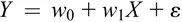
Regression models have a continuous response variable (often called a dependent variable). We will consider the case of a linear regression. Consider the case of a consumer products company that provides free samples to consumers to induce trial and also word-of-mouth to sell its products. Sometimes these companies may have their salespeople stationed at various retailers to distribute their samples in the hope that, after trying it, the consumers will like the product and purchase the product after their initial trial (“trial-and-repeat” purchase models in marketing). There is obviously some time lag between trial and repeat, and suppose the company wants to understand how their distribution of samples in a given month induces repeat purchases in the next month. We will denote the number of samples in a given month, say, October, as X and the number of repeat purchases in November by Y. We can treat the number of purchases Y as a continuous variable. Thus, Y is the continuous response variable and X is the explanatory (also called independent) variable. A simple model to predict Y based on X is

(1.1)

The epsilon term (ε) at the end is the error term. It captures the fact that the relationship between X and Y has randomness owing to a host of factors. The common sources of randomness are the many other factors that also affect purchases in November apart from trials in October. Of course, these have not been modeled, and thus, there will be errors when we use only one explanatory variable to predict purchases in November. In the simple linear regression above, the effect of the number of trial samples in October is given by the parameter w ₁ (parameters that multiply inputs are also called coefficients and in machine learning models like Neural Networks, they are called weights). The slope, given by w _1, intuitively captures the additional purchases in November due to an extra trial sample in October. The intercept, given by w ₀, intuitively captures the purchases in November if there were no trial samples in October (in machine learning models like Neural Networks this parameter is called the bias). Instead of just one explanatory variable, one could include other variables as well on the right-hand side of the equation, and then we would have a multiple regression.

In this book, we will refer to a model with a continuous response variable as a regression model and different machine learning techniques can be used to analyze such models. The traditional linear regression described above can serve as a useful benchmark to compare with the more recent machine learning models.

In marketing the response variable we are often interested in is categorical. For instance, consider the case of a bank that wants to predict whether its customers are likely to churn (leave) or not. A sales organization may be interested in categorizing their prospects as being either in the “buy” or “not buy” category. In lead scoring, a sales organization may want to categorize their sales leads as belonging to one of many different classes based on their propensities to buy: very unlikely, unlikely, likely, very likely. These are classification tasks, with the first two being binary classification and the third being multiclass classification.

We will briefly describe the case of binary classification. The traditional workhorse for analyzing models with a binary categorical response variable is a logistic regression. In the bank churn example, suppose the two classes are “churn” or “not churn,” and the bank wants to understand to what extent the amount of “balance” that the customer has is predictive of churn. The answer is not clear a priori. On the one hand, a customer with a large balance can be considered as having a deeper relationship with the bank, and therefore, less likely to churn. On the other hand, such attractive customers are targets of competitive offers from other banks and are more likely to churn. We use the balance a customer has in the bank as the explanatory variable X. The response variable Y = {+1, −1} is coded as: +1≡ “churn” and −1 ≡ “not churn.” We cannot use a linear regression here since we would like to model the probability of churning, and unlike the continuous response of a linear regression which can take on any value, probabilities have to lie in the interval [0, 1].

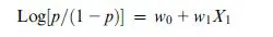
The logistic regression works by defining p = Probability(Y = +1), and then positing the relationship

(1.2)

The term on the left-hand side, Log[p/(1−p)], is called the log odds ratio. This formulation generates the probability of churning, p. It also ensures that the sum, Probability(“churn”) + Probability (“not churn”), adds up to 1 as is expected of probabilities. Based on these probabilities, one can classify customers as belonging to the category “churn” (“not churn”) if p > 0.5 (p < 0.5).

In this book, we will refer to a model with a categorical response variable, both binary and multiclass, as a classification model, and various machine learning models can be used for classification tasks. The logistic regression described above can serve as a benchmark to compare with machine learning classification models.

1.2 Cost Functions and Training of Machine Learning Models

Machine learning practitioners often talk of cost functions. Take the example of a company trying to predict sales of a certain product. Data are available over many past periods, and in each period, sales are affected by factors like the company's own price, advertising spending, and the competitor's prices among other factors. Given this situation, we want to accurately predict the sales of the company. One way to do this is to create a mathematical formulation (model) that allows us to predict sales based on observed factors (like price, advertising, etc.) for each recorded period in the past. Then, we can compare the actual past sales value against the sales value predicted by this model to see how well the model is performing. In this case, the cost function is a function of the difference between the predicted output of the model and the actual sales value for all past periods. The model is said to perform well when the cost (also called error or loss) is minimized. The minimization of cost is achieved by choosing appropriate parameters of the mathematical model. This process is called training the machine learning model.

For a machine learning model, training is said to occur when the model estimates the “best” values of the parameters. What does best mean? At this point, we formalize the concept of a cost function a bit more. Consider the linear regression model specified above. Given a specific input data point, X = x, and some values of the parameters (weights), the regression model can make a prediction f (x). ¹ This is, given specific values of w ₀ and w ₁ and a data point x, the regression model makes a prediction

= f (x) = w₀ +w₁x. On the other hand, the input data point x has an actual observed y (also called target) associated with it. Intuitively, the cost function measures the discrepancy between the model prediction

and the actual y for all possible values of input x. The goal of training is to choose those parameters (weights w₀ and w₁) that minimize this cost. These cost minimizing weights are the “best” weights.

In our discussions earlier, the cost function was based on sales – specifically it was the difference between actual observed sales and the sales predicted by the model. In business, typical “performance indicators...