Calculus of Variations and Optimal Control Theory

A Concise Introduction

Daniel Liberzon

• Publisher: Princeton University Press
• Year: 2011
• ISBN:
  9781400842643
• Topic: Mathematics
• Subtopic: Applied Mathematics
• Index: Mathematics

This textbook offers a concise yet rigorous introduction to calculus of variations and optimal control theory, and is a self-contained resource for graduate students in engineering, applied mathematics, and related subjects. Designed specifically for a one-semester course, the book begins with calculus of variations, preparing the ground for optimal control. It then gives a complete proof of the maximum principle and covers key topics such as the Hamilton-Jacobi-Bellman theory of dynamic programming and linear-quadratic optimal control. Calculus of Variations and Optimal Control Theory also traces the historical development of the subject and features numerous exercises, notes and references at the end of each chapter, and suggestions for further study.

• Offers a concise yet rigorous introduction
• Requires limited background in control theory or advanced mathematics
• Provides a complete proof of the maximum principle
• Uses consistent notation in the exposition of classical and modern topics
• Traces the historical development of the subject
• Solutions manual (available only to teachers)

Leading universities that have adopted this book include:

• University of Illinois at Urbana-Champaign ECE 553: Optimum Control Systems
• Georgia Institute of Technology ECE 6553: Optimal Control and Optimization
• University of Pennsylvania ESE 680: Optimal Control Theory
• University of Notre Dame EE 60565: Optimal Control

Chapter One

Introduction

1.1 OPTIMAL CONTROL PROBLEM

We begin by describing, very informally and in general terms, the class of optimal control problems that we want to eventually be able to solve. The goal of this brief motivational discussion is to fix the basic concepts and terminology without worrying about technical details.

The first basic ingredient of an optimal control problem is a control system. It generates possible behaviors. In this book, control systems will be described by ordinary differential equations (ODEs) of the form

(1.1)

where x is the state taking values in Rⁿ, u is the control input taking values in some control set

, t is time, t₀ is the initial time, and x₀ is the initial state. Both x and u are functions of t, but we will often suppress their time arguments.

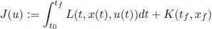
The second basic ingredient is the cost functional. It associates a cost with each possible behavior. For a given initial data (t₀,x₀), the behaviors are parameterized by control functions u. Thus, the cost functional assigns a cost value to each admissible control. In this book, cost functionals will be denoted by J and will be of the form

(1.2)

where L and K are given functions (running cost and terminal cost, respectively), t_f is the final (or terminal) time which is either free or fixed, and x_f := x(t_f ) is the final (or terminal) state which is either free or fixed or belongs to some given target set. Note again that u itself is a function of time; this is why we say that J is a functional (a real-valued function on a space of functions).

The optimal control problem can then be posed as follows: Find a control u that minimizes J(u) over all admissible controls (or at least over nearby controls). Later we will need to come back to this problem formulation and fill in some technical details. In particular, we will need to specify what regularity properties should be imposed on the function f and on the admissible controls u to ensure that state trajectories of the control system are well defined. Several versions of the above problem (depending, for example, on the role of the final time and the final state) will be stated more precisely when we are ready to study them. The reader who wishes to preview this material can find it in Section 3.3.

It can be argued that optimality is a universal principle of life, in the sense that many—if not most—processes in nature are governed by solutions to some optimization problems (although we may never know exactly what is being optimized). We will soon see that fundamental laws of mechanics can be cast in an optimization context. From an engineering point of view, optimality provides a very useful design principle, and the cost to be minimized (or the profit to be maximized) is often naturally contained in the problem itself. Some examples of optimal control problems arising in applications include the following:

• Send a rocket to the moon with minimal fuel consumption.

• Produce a given amount of chemical in minimal time and/or with minimal amount of catalyst used (or maximize the amount produced in given time).

• Bring sales of a new product to a desired level while minimizing the amount of money spent on the advertising campaign.

• Maximize throughput or accuracy of information transmission over a communication channel with a given bandwidth/capacity.

The reader will easily think of other examples. Several specific optimal control problems will be examined in detail later in the book. We briefly discuss one simple example here to better illustrate the general problem formulation.

Example 1.1 Consider a simple model of a car moving on a horizontal line. Let

be the car’s position and let u be the acceleration which acts as the control input. We put a bound on the maximal allowable acceleration by letting the control set U be the bounded int...