Lessons from Nanoelectronics

A New Perspective on Transport

Supriyo Datta

• Publisher: WSPC
• Year: 2012
• ISBN:
  9789814483902
• Topic: Scienze fisiche
• Subtopic: Fisica

Everyone is familiar with the amazing performance of a modern smartphone, powered by a billion-plus nanotransistors, each having an active region that is barely a few hundred atoms in length.

These lecture notes are about a less appreciated by-product of the microelectronics revolution, namely the deeper understanding of current flow, and device operation that it has enabled, which forms the basis for a new approach to transport problems.

The book assumes very little background beyond linear algebra and differential equations, and is intended to be accessible to anyone in any branch of science or engineering.

Readers are encouraged to visit the website http://nanohub.org/groups/lnebook to access revisions, corrections, video lectures, tutorials, quizzes and also to join a Q&A forum based on questions from readers.

Contents:

• The New Ohm's Law:
  • The Bottom-Up Approach
  • Why Electrons Flow
  • The Elastic Resistor
  • Ballistic and Diffusive Transport
  • Conductivity
  • Diffusion Equation for Ballistic Transport
  • What about Drift?
  • Electrostatics is Important
  • Smart Contacts
• Old Topics in New Light:
  • Thermoelectricity
  • Phonon Transport
  • Measuring Electrochemical Potentials
  • Hall Effect
  • Spin Valve
  • Kubo Formula
  • Second Law
  • Fuel Value of Information
• Contact-ing Schrödinger:
  • The Model
  • Non-Equilibrium Green's Functions (NEGF)
  • Can Two Offer Less Resistance than One?
  • Quantum of Conductance
  • Rotating an Electron
  • Does NEGF Include “Everything”?
  • The Quantum and the Classical

Readership: Students and professionals in any branch of science or engineering.

III. Contact-ing Schrdinger

18. The Model

19. NEGF Method

20. Can Two Offer Less Resistance than One?

21. Quantum of Conductance

22. Rotating an Electron

23. Does NEGF Include “Everything?”

24. The Quantum and the Classical

Lecture 18

The Model

18.1. Schrödinger Equation

18.2. Electron-Electron Interactions

18.3. Differential to Matrix Equation

18.4. Choosing Matrix Parameters

Over a century ago Boltzmann taught us how to combine Newtonian mechanics with entropy-driven processes

and the resulting Boltzmann transport equation (BTE) is widely accepted as the cornerstone of semiclassical transport theory. Most of the results we have discussed so far can be (and generally are) obtained from the Boltzmann equation, but the concept of an elastic resistor makes them more transparent by spatially separating force-driven processes in the channel from the entropy-driven processes in the contacts.

In this part of these lecture notes I would like to discuss the quantum version of this problem, using the non-equilibrium Green’s function (NEGF) method to combine quantum mechanics described by the Schrödinger equation with "contacts"

much as Boltzmann taught us how to combine classical dynamics with "contacts".

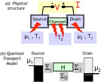
Fig.18.1. (a) Generic device structure that we have been discussing. (b) General quantum transport model with elastic channel described by a Hamiltonian [H] and its connection to each ‘contact” described by a corresponding self-energy [Σ].

The NEGF method originated from the classic works in the 1960’s that used the methods of many-body perturbation theory to describe the distributed entropy-driven processes along the channel. Like most of the work on transport theory (semiclassical or quantum) prior to the 1990’s, it was a “contact-less” approach focused on the interactions occurring throughout the channel, in keeping with the general view that the physics of resistance lay essentially in these distributed entropy generating processes.

As with semiclassical transport, our bottom-up perspective starts at the other end with the elastic resistor with entropy-driven processes confined to the contacts. This makes the theory less about interactions and more about "connecting contacts to the Schrödinger equation", or more simply, about contact-ing Schrödinger.

But let me put off talking about the NEGF model till the next Lecture, and use subsequent lectures to illustrate its application to interesting problems in quantum transport. As indicated in Fig.18.1b the NEGF method requires two types of inputs: the Hamiltonian, [H] describing the dynamics of an elastic channel, and the self-energy [Σ]describing the connection to the contacts, using the word “contacts” in a broad figurative sense to denote all kinds of entropy-driven processes. Some of these contacts are physical like the ones labeled “1” and “2” in Fig.18.1b, while some are conceptual like the one labeled “0” representing entropy changing processes distributed throughout the channel.

In this Lecture let me just try to provide a super-brief but self-contained introduction to how one writes down the Hamiltonian [H]. The [Σ] can be obtained by imposing the appropriate boundary conditions and will be described in later Lectures when we look at specific examples applying the NEGF method.

We will try to describe the procedure for writing down [H] so that it is accessible even to those who have not had the benefit of a traditional multi-semester introduction to quantum mechanics. Moreover, our emphasis here is on something that may be helpful even for those who have this formal background. Let me explain.

Most people think of the Schrödinger equation as a differential equation which is the form we see in most textbooks. However, practical calculations are usually based on a discretized version that represents the differential equation as a matrix equation involving the Hamiltonian matrix [H] of size NxN, N being the number of “basis functions” used to represent the structure.

This matrix [H] can be obtained from first principles, but a widely used approach is to represent it in terms of a few parameters which are chosen to match key experiments. Such semi-empirical approaches are often used because of their convenience and because they can often explain a wide range of experiments beyond the key ones that are used as input, suggesting that they capture a lot of essential physics.

In order to follow the rest of the Lectures it is important for the readers to get a feeling for how one writes down this matrix [H] given an a...