Path Integrals for Pedestrians

Ennio Gozzi, Enrico Cattaruzza, Carlo Pagani

• Éditeur: WSPC
• Année: 2015
• ISBN:
  9789814603959
• Sujet: Physical Sciences
• Sous-sujet: Physics

This is a book on path integrals which provides a quick and swift description of the topic. It contains original material that never before has appeared in a book. The new topics include the path integrals for the Wigner functions and for Classical Mechanics.

Request Inspection Copy

This is a book on path integrals which provides a quick and swift description of the topic. It contains original material that never before has appeared in a book. The new topics include the path integrals for the Wigner functions and for Classical Mechanics.

Request Inspection Copy

Readership: Student and professional in quantum and classical mechanics.
Key Features:

• Work-out problems for students
• Path integral for classical mechanics
• Path integral for Wigner functions

Chapter 1

The Basic Ideas

1.1Quantum mechanics and summing up amplitudes

The path integral approach to quantum mechanics was developed by R. F. Feynman in his Ph.D. thesis of 1942. It was later published (1948) in Rev. Mod. Phys. with the title “Space-time approach to non-relativistic Quantum Mechanics” [Feynman (1948)].

Feynman wanted a formulation of quantum mechanics in which “space-time” played a role and not just the Hilbert space, like in the traditional version of quantum mechanics. His approach is very helpful in “visualizing” many quantum mechanical phenomena and in developing various techniques, like the Feynman diagrams, the non-perturbative methods (

→ 0, N → ∞), etc. Somehow, Dirac [Dirac (1933)] had got close to the Feynman formulation of quantum mechanics in a paper in which he asked himself what is the role of the Lagrangian in quantum mechanics.

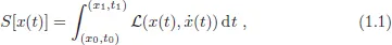
Let us first review the concept of action which everybody has learned in classical mechanics. Its definition is

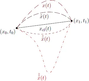
where x(t) is any trajectory between (x₀ , t₀) and (x₁ , t₁), not necessarily the classical one, and

is the Lagrangian of the system. The action S[x(t)] is what in mathematical terms is known as a functional. Remember that a functional is a map between a space of functions x(t) and a set of numbers (the real or complex numbers). From Eqn.(1.1) one sees that S[x(t)] is a functional because, once we insert the function x(t) on the right-hand side of Eqn.(1.1) (and perform the integration), we get a real number which is the value of the action on that trajectory. If we change the trajectory, we get a different number.

Fig. 1.1

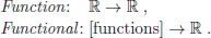
A functional is indicated with square brackets, S[x(t)], differently from a function whose argument is indicated with round brackets: f(x). A function f(x) is a map between the set of numbers (real, complex, etc.) and another set of numbers (real, complex, etc.). So, if we restrict to the real numbers, we can say that:

Given these definitions, let us now see what the path integral formulation of quantum mechanics given by Feynman is.

We know that in quantum mechanics a central element is the transition kernel to go from (x₀ , t₀) to (x₁, t₁) which is defined as

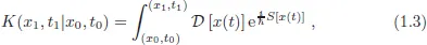
What Feynman proved is the following formula:

where, on the right-hand side of Eqn.(1.3), the symbol

indicates a functional integration which “roughly” consists of the sum over all trajectories between (x₀ , t₀) and (x₁, t₁).

So, in Eqn.(1.3) we insert a trajectory in

calculate this quantity and “sum” it to the same expression with a different trajectory and so on for all trajectories between (x₀, t₀) and (x₁, t₁). This is the reason why this method is called path integral. Note that all trajectories enter Eqn.(1.3) and not just the classical one.

1.2Double slit experiment

We shall give a rigorous derivation of Eqn.(1.3) but for the moment let us try to grasp a “more physical” reason of why trajectories enter the expression of the quantum transition kernel. This part is taken from the book [Feynman and Hibbs (1965)].

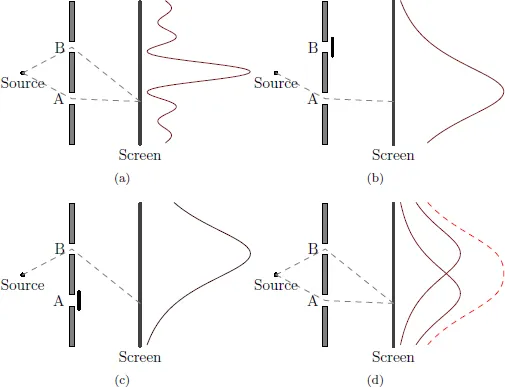
Let us recall the double slit experiment, see Fig. 1.2.

Fig. 1.2 (a) The probability P_AB with both slits open. (b) The probability P_A obtained with only the slit A open. (c) The probability PB obtained keeping only the slit B open. (d) Note that P_AB ≠ P_A + P_B.

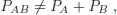
In Fig. 1.2(a) both slits A and B are open while in the other two figures, 1.2(b) and 1.2(c) only one is open. It is well known that the probabilities P_AB , P_A, P_B satisfy the inequality

while for the probability amplitudes ψ_AB , ψ_A , ψ_B we have

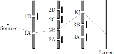
Let us now put more screens with different openings, like in Fig. 1.3.

Fig. 1.3 More screens with different openings.

Let us suppose we close the slits 1B, 2A, 2C, 2D, 3A, 3B and let us call the associated wave function as

where we have indicated with a subindex in the wave functions the slits which are open. For example for the wave function above only the slits 1A, 2B and 3C are open as shown in Fig. 1.3.

We can “associate” this amplitude with the path...