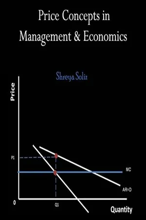
Economics
Marginal Cost
Marginal cost refers to the additional cost incurred by producing one more unit of a good or service. It is calculated by dividing the change in total cost by the change in quantity produced. Understanding marginal cost is crucial for businesses to make decisions about production levels and pricing strategies, as it helps determine the most efficient allocation of resources.
Written by Perlego with AI-assistance
Related key terms
1 of 5
10 Key excerpts on "Marginal Cost"
 No longer available |Learn more
- (Author)
- 2014(Publication Date)
- Orange Apple(Publisher)
Note that the Marginal Cost will change with volume, as a non-linear and non-proportional cost function includes • variable terms dependent to volume, • constant terms independent to volume and occurring with the respective lot size, • jump fix cost increase or decrease dependent to steps of volume increase. So at each level of production, the Marginal Cost is the cost of the next unit produced referring to the basic volume. ____________________ WORLD TECHNOLOGIES ____________________ In general terms, Marginal Cost at each level of production includes any additional costs required to produce the next unit. If producing additional vehicles requires, for example, building a new factory, the Marginal Cost of those extra vehicles includes the cost of the new factory. In practice, the analysis is segregated into short and long-run cases, and over the longest run, all costs are marginal. At each level of production and time period being considered, Marginal Costs include all costs which vary with the level of production, and other costs are considered fixed costs. A number of other factors can affect Marginal Cost and its applicability to real world problems. Some of these may be considered market failures. These may include information asymmetries, the presence of negative or positive externalities, transaction costs, price discrimination and others. Cost functions and relationship to average cost In the simplest case, the total cost function and its derivative are expressed as follows, where Q represents the production quantity, VC represents variable costs, FC represents fixed costs and TC represents total costs. Since (by definition) fixed costs do not vary with production quantity, it drops out of the equation when it is differentiated. The important conclusion is that Marginal Cost is not related to fixed costs. This can be compared with average total cost or ATC, which is the total cost divided by the number of units produced and does include fixed costs. eBook - PDF
- Irvin Tucker(Author)
- 2018(Publication Date)
- Cengage Learning EMEA(Publisher)
7–2b The Marginal Revenue Equals Marginal Cost Method A second approach uses marginal analysis to determine the profit-maximizing level of output by comparing marginal revenue (marginal benefit) and Marginal Cost. Recall from the previous chapter that a synonym for marginal is “extra” and that Marginal Cost is the change in total cost as the output level increases by one unit. Also recall that these Marginal Cost data are listed between the quantity of output line entries because the change in total cost occurs between each additional whole unit of output rather than exactly at each listed output level. Now we introduce marginal revenue (MR), a concept similar to Marginal Cost. Marginal revenue is the “extra” revenue or the change in total revenue from the sale of one additional unit of output. Stated another way, marginal revenue is the ratio of the change in total revenue to a change in output. Marginal revenue (MR) The change in total revenue from the sale of one additional unit of output. Copyright 2019 Cengage Learning. All Rights Reserved. May not be copied, scanned, or duplicated, in whole or in part. Due to electronic rights, some third party content may be suppressed from the eBook and/or eChapter(s). Editorial review has deemed that any suppressed content does not materially affect the overall learning experience. Cengage Learning reserves the right to remove additional content at any time if subsequent rights restrictions require it. eBook - ePub
- Arleen J Hoag, John H Hoag(Authors)
- 2006(Publication Date)
- WSPC(Publisher)
Chapter 10 COST Key Topics total cost implicit cost average total cost Marginal Cost the average-marginal relation Goals understand how costs behave and why understand how cost concepts are related relate Marginal Cost to marginal product and diminishing returns Your first introduction to cost was opportunity cost in Chapter 1. Opportunity costs are always present in decision making. In the case of the firm, one opportunity cost is the cost of producing output. The cost of production is the subject of this chapter. Cost is important since it is part of the information the firm needs to decide the amount of output to supply. Supply, together with demand, determines price and how resources are allocated in a market. When you have completed this chapter, you will have an understanding of how cost behaves when output changes. An important lesson from the study of cost is that different costs follow predictable patterns. One thing you will learn is what the patterns are and another is what causes the patterns. Different cost concepts answer different questions for the firm, so we will break cost down into three different groups. These groups are total cost, average cost, and Marginal Cost. Total Cost Your study of cost begins with the group of total cost. The total cost group is composed of three cost concepts: total fixed cost, total variable cost, and total cost. These will be discussed starting with total fixed cost. Total fixed cost (TFC) is the cost that does not change with the level of output. This means that the total fixed cost remains the same, or constant, whether zero or an infinite amount of output is produced. Fixed cost is not related to the level of production. Fixed cost occurs because in the short run, there is at least one factor that cannot be changed. The cost of the fixed factor is the fixed cost. The cost of this factor does not depend on the level of output produced because the amount of the factor, and therefore its cost, remains unchanged eBook - PDF
- James D Gwartney, Richard Stroup, J. R. Clark(Authors)
- 2014(Publication Date)
- Academic Press(Publisher)
The irrelevance of sunk costs helps to explain why it often makes sense to continue operating older equipment (it has a low opportunity cost), even though it might not be wise to purchase similar equipment again. Costs and Supply Economists are interested in cost because they seek to explain the supply decisions of firms. A strictly profit-maximizing firm will compare the expected revenues derived from a decision or a course of action with the expected costs. If the expected revenues exceed costs, the course of action will be chosen be-cause it will expand profits (or reduce losses). In the short run, the Marginal Cost of producing additional units is the relevant cost consideration. A profit-maximizing decision-maker will compare the expected Marginal Costs with the expected additional revenues from larger sales. If the latter exceeds the former, output (the quantity supplied) will be expanded. Whereas Marginal Costs are central to the choice of short-run output, the expected average total cost is vital to a firm's long-run supply decision. Before entry into an industry, a profit-maximizing decision-maker will compare the ex-pected market price with the expected long-run average total cost. Profit-seeking potential entrants will supply the product if, and only if, they expect the market price to exceed their long-run average total cost. Similarly, existing firms will continue to supply a product only if they expect the market price to enable them at least to cover their long-run average total cost. CHAPTER 13 COSTS AND THE SUPPLY OF GOODS 3 0 3 LOOKING AHEAD In this chapter, we outlined several basic principles that affect costs for business firms. W e will use these basic principles w h e n we analyze the price a n d o u t p u t decisions of firms u n d e r alternative market structures in the chapters t h a t follow. CHAPTER LEARNING l The business firm is used to organize productive resources and transform them into OBJECTIVES goods and services. eBook - ePub
- David Horner(Author)
- 2020(Publication Date)
- Kogan Page(Publisher)
Note that we are now talking about variable cost of production. In effect, this is the same as the direct costs of production – those which vary directly with the level of production. Direct costs can be thought of as those which are related to a particular product or cost unit. Variable costs are, more generally, those costs relating to overall level of output. Within the Marginal Costing approach, the distinction between variable cost and direct cost is not critical and often these terms will be used interchangeably.Uses of Marginal Costing
In the long term, all costs are, in effect, variable as the firm can always decide to close down and therefore would not incur any costs at all – fixed or variable. However, although the fixed costs will still have to be paid in the short term, the firm will have control over the variable costs and can either increase or decrease these by making decisions about production levels. Marginal Costing focuses on short-term decisions and looks at the effects of these decision on revenue and variable costs of production.There are a number of situations where the Marginal Costing approach will provide more useful information for decision making than the absorption costing approach. Situations where Marginal Costing proves useful would include the following:- break-even analysis;
- devising an optimum production plan where resources are limited;
- deciding whether to make a product or to buy in the product instead;
- accepting an order at lower than the normal selling price;
- closing down either a branch or a segment of the business.
Break-even analysis
A firm will break-even if its total revenue is equal to total costs. If revenue exceeds the total level of costs, a profit will be generated, and if revenue is lower than total costs, a loss will be generated. However, breaking even is often seen as an important stepping stone for businesses, especially in their early years when struggling to survive might be more important than earning substantial profits. As long as a firm can avoid making losses, breaking even is often seen as a bare-minimum target to be aimed for. In this case, the level of sales or output needed in order to achieve this break-even level will be useful knowledge. eBook - PDF
Campus Economics
How Economic Thinking Can Help Improve College and University Decisions
- Sandy Baum, Michael McPherson(Authors)
- 2023(Publication Date)
- Princeton University Press(Publisher)
Does this mean that the college should not accept a student from whom it cannot collect $20,000 of tuition unless it is making a conscious decision to take a loss on the student to provide broader opportunity or diversity in the student body or in some other way to obtain a specific benefit? No. The relevant concept for making this decision is Marginal Cost. Marginal Cost is the change in total cost that results from producing one more unit—in this case from enrolling one additional student. The Marginal Cost of additional students is frequently much lower than the average cost. Once the classrooms and dormitories are built and the faculty hired, an extra Basic economic concepts [ 33 ] student doesn’t add much to the cost of operation. There is a limit to this of course. If the college decides to enroll two hundred addi- tional students, it will probably have to hire additional personnel and expand facilities. But for most institutions, the Marginal Cost of a few extra students is quite low. The marginal/average contrast explains, for example, why airlines sell seats at low fares if they think they will not otherwise be filled. Once the plane is flying, the Marginal Cost of additional passengers is very low. If the total cost of flying an airliner with a capacity of 500 passengers is $350,000, the airline will lose money if it doesn’t charge an average of at least $700 per person. But it makes sense to let an extra person come on board at the last minute even if he is willing to pay much less than this—just enough to cover any extra fuel cost resulting from the additional weight. To determine whether the school’s financial situation will improve with the enrollment of a student who pays, say, $3,000 in tuition, the relevant question is whether $3,000 covers the mar- ginal cost of educating the student. Does the student add more to revenues than she does to costs? If so, from a purely short-term financial perspective, the student should be enrolled. eBook - PDF
Managerial Economics
Problem-Solving in a Digital World
- Nick Wilkinson(Author)
- 2022(Publication Date)
- Cambridge University Press(Publisher)
We can now examine these effects as they relate to the various forms of production function described in (6.2) to (6.7). First we need to explain more precisely the economic interpretation of marginal effects in the context of production theory. A marginal effect is given mathematically by a derivative, or, more precisely, in the case of the two-input production function, a partial derivative (obtained by differentiating the production function with respect to one variable, while keeping other variables constant). The economic interpretation of this is a marginal product. The marginal product of labour is the additional output resulting from using one more unit of labour, while holding the capital input constant. Likewise, the marginal product of capital is the additional output resulting from using one more unit of capital, while holding the labour input constant. These marginal products can thus be expressed mathematically in terms of the following partial derivatives: Table 6.1 Input–output table for cubic function – Viking Shoes Capital input (machines) K 1 2 3 4 5 6 7 8 Labour input (workers) L 1 4 9 13 18 23 27 31 35 2 8 17 27 36 45 54 62 70 3 12 26 39 53 67 80 B 92 102 4 16 33 50 68 85 102 117 131 5 18 38 59 80 C 100 A 119 137 153 6 20 42 64 87 110 131 150 167 7 20 43 66 90 113 135 155 171 8 19 41 64 87 110 131 149 164 282 6 Production Theory MP L ¼ ∂Q=∂L and MP K ¼ ∂Q=∂K: Expressions for marginal product can now be derived for each of the mathematical forms (6.2) to (6.7). These are shown in Table 6.2, in terms of the marginal product of labour. The marginal product of capital will have the same general form because of the symmetry of the functions. The linear production function has constant marginal product, meaning that the marginal product is not affected by the level of either the labour or the capital input. This is not normally a realistic situation, and such functions, in spite of their simplicity, are not frequently used. eBook - PDF
Economics
Principles & Policy
- William Baumol, Alan Blinder, John Solow, , William Baumol, Alan Blinder, John Solow(Authors)
- 2019(Publication Date)
- Cengage Learning EMEA(Publisher)
The “law” of diminishing marginal returns crops up a lot in ordinary life— not just in the world of business. Consider Jason and his study habits: He has a tendency to procrastinate and then cram for exams the night before he takes them, pulling “all-nighters” regularly. How might an economist compare Jason’s marginal reward from an additional hour of study in the wee hours of the morning, relative to that of Colin, who studies for two hours every night? Closer to Home: The Diminishing Marginal Returns to Studying Bill Varie/Alamy Stock Photo Copyright 2020 Cengage Learning. All Rights Reserved. May not be copied, scanned, or duplicated, in whole or in part. Due to electronic rights, some third party content may be suppressed from the eBook and/or eChapter(s). Editorial review has deemed that any suppressed content does not materially affect the overall learning experience. Cengage Learning reserves the right to remove additional content at any time if subsequent rights restrictions require it. Chapter 7 Production, Inputs, and Cost: Building Blocks for Supply Analysis 133 7-3 MULTIPLE INPUT DECISIONS: THE CHOICE OF OPTIMAL INPUT COMBINATIONS 4 Up to this point we have simplified our analysis by assuming that the firm can change the quantity of only one of its inputs and that the price the product can command does not change, no matter how large a quantity the producer offers for sale (the fixed price is $15,000 for Al’s garages). Of course, neither of these assumptions is true in reality. In Chapter 8, we will explore the effect of product quantity decisions on prices by bringing in the demand curve. First, we must deal with the obvious fact that a firm must decide on the quantities of each of the many inputs it uses, not just one input at a time. That is, Al must decide not only how many carpenters to hire but also how much lumber and how many tools to buy. Both of the latter decisions clearly depend on the number of carpenters in his team. eBook - PDF
Microeconomics
Private and Public Choice
- James Gwartney, Richard Stroup, Russell Sobel, David Macpherson(Authors)
- 2017(Publication Date)
- Cengage Learning EMEA(Publisher)
While Marginal Costs are central in the short run, average total costs are the rele- vant cost consideration in the long run. Before entering an industry (or purchasing capital assets for expansion or replacement), a profit-maximizing decision-maker will compare the expected market price with the expected long-run average total cost. Profit-seeking poten- tial entrants will supply the product if, and only if, they expect the market price to exceed their long-run average total cost. Similarly, existing firms will continue to supply a product in the long run only if they expect that the market price will enable them at least to cover their long-run average total cost. LOOKINGuni00A0AHEAD Copyright 2018 Cengage Learning. All Rights Reserved. May not be copied, scanned, or duplicated, in whole or in part. WCN 02-300 CHAPTER 8 COSTS AND THE SUPPLY OF GOODS 171 • The business firm is used to organize productive resources and trans- form them into goods and services. There are three major types of business structure—proprietorships, partnerships, and corporations. • The principal–agent problem tends to reduce efficiency within the firm. Monitoring and the structure of incentives can be used to minimize inefficiencies arising from this source. • The demand for a product indicates the intensity of consumers’ desires for the item. The (opportunity) cost of producing the item indicates the intensity of consumers’ desires for other goods that could have been produced instead, with the same resources. • In economics, total cost includes not only explicit payments for resources employed by the firm, but also the implicit costs asso- ciated with the use of productive resources owned by the firm (like the opportunity cost of the firm’s equity capital or owner- provided services) that could be used elsewhere. eBook - PDF
Economics
A Contemporary Introduction
- William A. McEachern(Author)
- 2016(Publication Date)
- Cengage Learning EMEA(Publisher)
A firm with total revenues of $125 million, explicit costs of $100 million, and implicit costs of $30 million c. A firm with total revenues of $100 million, explicit costs of $90 million, and implicit costs of $20 million d. A firm with total revenues of $250,000, explicit costs of $275,000, and implicit costs of $50,000 4. Alternative Measures of Profit Why is it reasonable to think of normal profit as a type of cost to the firm? 5. Short Run Versus Long Run What distinguishes a firm’s short- run period from its long-run period? 6. Law of Diminishing Marginal Returns As a farmer, you must decide how many times during the year to plant a new crop. Also, you must decide how far apart to space the plants. Will diminishing returns be a factor in your decision making? If so, how will it affect your decisions? 7. Marginal Cost What is the difference between fixed cost and variable cost? Does each type of cost affect short-run Marginal Cost? If yes, explain how each affects Marginal Cost. If no, explain why each does or does not affect mar- ginal cost. 8. Marginal Cost Explain why the Marginal Cost of production must increase if the marginal product of the variable resource is decreasing. 9. Costs in the Short Run What effect would each of the follow- ing have on a firm’s short-run Marginal Cost curve and its fixed cost curve? a. An increase in the wage rate b. A decrease in property taxes c. A rise in the purchase price of new capital d. A rise in energy prices 10. Costs in the Short Run Identify each of the curves in the fol- lowing graph: Cost per unit Quantity C B A 11. Marginal Cost and Average Cost Explain why the Marginal Cost curve must intersect the average total cost curve and the average variable cost curve at their minimum points. Why do the average total cost curve and average variable cost curve get closer to one another as output increases? 12.
Index pages curate the most relevant extracts from our library of academic textbooks. They’ve been created using an in-house natural language model (NLM), each adding context and meaning to key research topics.