Inverse Hyperbolic Functions

10 Key excerpts on "Inverse Hyperbolic Functions"

• 

  eBook - PDF

  The Calculus Lifesaver

  All the Tools You Need to Excel at Calculus

  • Adrian Banner(Author)
  • 2009(Publication Date)
  • Princeton University Press

    (Publisher)

  If you want an inverse for this function, you have to throw away the left half of the graph, just as you do when you take the positive square root (and throw away the negative one). On the other Section 10.3: Inverse Hyperbolic Functions • 221 hand, y = sinh( x ) already satisfies the horizontal line test, so there’s nothing that needs to be done. So we get two inverse functions with the following properties: cosh -1 is neither odd nor even; it has domain [1 , ∞ ) and range [0 , ∞ ). sinh -1 is odd; its domain and range are all of R . The graphs are obtained by reflecting the original graphs in the line y = x as usual: 1 y = cosh -1 ( x ) y = sinh -1 ( x ) The derivatives are obtained in the same way that we got the derivatives of the inverse trig functions. In particular, if y = cosh -1 ( x ), then x = cosh( y ); differentiating implicitly with respect to x , we get 1 = sinh( y ) dy dx . (Remember that the derivative of cosh( x ) with respect to x is sinh( x ), not -sinh( x ).) Now cosh 2 ( y ) -sinh 2 ( y ) = 1, so we can rearrange and take square roots to see that sinh( y ) = ± q cosh 2 ( y ) -1 = ± √ x 2 -1. Since cosh -1 ( x ) is clearly increasing in x , we end up with d dx cosh -1 ( x ) = 1 √ x 2 -1 for x > 1 . In exactly the same way, you should be able to check that d dx sinh -1 ( x ) = 1 √ x 2 + 1 for all real x. Now, let’s forget about the calculus for a few seconds and recall the definitions of cosh( x ) and sinh( x ): cosh( x ) = e x + e -x 2 and sinh( x ) = e x -e -x 2 . Since we can write cosh( x ) and sinh( x ) in terms of exponentials, we should be able to write the inverse functions in terms of logarithms. After all, exponen-tials and logarithms are inverses of each other. Let’s see how it works. For example, if y = cosh -1 ( x ), then x = cosh( y ) = ( e y + e -y ) / 2. Now you can 222 • Inverse Functions and Inverse Trig Functions solve for y by using a little trick.

  Sign up to read

  Learn more about book
• 

  eBook - ePub

  Engineering Mathematics

  A Programmed Approach, 3th Edition

  • C W. Evans, C. Evans(Authors)
  • 2019(Publication Date)
  • CRC Press

    (Publisher)

  Hyperbolic functions 5

  Although we have now explored some of the basic terminology of mathematics and developed the techniques of the differential calculus, we need to pause to extend our algebraic knowledge. In this chapter we shall describe a class of functions known as the hyperbolic functions which are very similar in some ways to the circular functions. We shall use the opportunity to consider in detail what is meant by an inverse function.

  After studying this chapter you should be able to □  Use the hyperbolic functions and their identities; □  Solve algebraic equations which involve hyperbolic functions; □  Differentiate hyperbolic functions; □  Decide when a function has an inverse function; □  Express Inverse Hyperbolic Functions in logarithmic form. We shall also consider a practical problem concerning the sag of a chain. 5.1      DEFINITIONS AND IDENTITIES

  The hyperbolic functions are in some ways very similar to the circular functions. Indeed when we deal with complex numbers (Chapter 10 ) we shall see that there is an algebraic relationship between the two. Initially we shall discuss the hyperbolic functions algebraically, but later we shall see that one of them arises in a physical context.

  The functions cosine and sine are called circular functions because x = cos θ and y = sin θ satisfy the equation x2 + y2 = 1, which is the equation of a circle. The functions known as the hyperbolic cosine (cosh) and the hyperbolic sine (sinh) are called hyperbolic functions because x = cosh u and y = sinh u satisfy the equation x2 – y2 = 1, which is the equation of a rectangular hyperbola.

  We shall define the hyperbolic functions and use these definitions to sketch their graphs. Here then are the definitions:

  Sign up to read

  Learn more about book
• 

  eBook - PDF

  Single Variable Calculus, Metric Edition

  • James Stewart, Daniel K. Clegg, Saleem Watson, , James Stewart, James Stewart, Daniel K. Clegg, Saleem Watson(Authors)
  • 2020(Publication Date)
  • Cengage Learning EMEA

    (Publisher)

  y 0 x y=_1 y=1 1 2 y= ´ y=_ e–® 1 2 y=sinh x 0 y x y= e–® 1 2 1 2 y= ´ y=cosh x 1 0 y x FIGURE 1 y - sinh x - 1 2 e x 2 1 2 e 2x FIGURE 2 y - cosh x - 1 2 e x 1 1 2 e 2x FIGURE 3 y - tanh x Note that sinh has domain R and range R, whereas cosh has domain R and range f1, `d. The graph of tanh is shown in Figure 3. It has horizontal asymptotes y - 61. (See Exercise 27.) Some of the mathematical uses of hyperbolic functions will be seen in Chapter 7. Applications to science and engineering occur whenever an entity such as light, velocity, electricity, or radioactivity is gradually absorbed or extinguished because the decay can be represented by hyperbolic functions. The most famous application is the use of hyper- bolic cosine to describe the shape of a hanging wire. It can be proved that if a heavy flexible cable (such as an overhead power line) is suspended between two points at the same height, then it takes the shape of a curve with equation y - c 1 a coshs x y ad called a catenary (see Figure 4). (The Latin word catena means “chain.”) Another application of hyperbolic functions occurs in the description of ocean waves: the velocity of a water wave with length L moving across a body of water with depth d is modeled by the function v - Î tL 2 tanh S 2d L D where t is the acceleration due to gravity (see Figure 5 and Exercise 57). The hyperbolic functions satisfy a number of identities that are similar to well-known trigonometric identities. We list some of them here and leave most of the proofs to the exercises. y 0 x FIGURE 4 A catenary y - c 1 a coshs xyad d L FIGURE 5 Idealized water wave Copyright 2021 Cengage Learning. All Rights Reserved. May not be copied, scanned, or duplicated, in whole or in part. Due to electronic rights, some third party content may be suppressed from the eBook and/or eChapter(s). Editorial review has deemed that any suppressed content does not materially affect the overall learning experience.

  Sign up to read

  Learn more about book
• 

  eBook - PDF

  Calculus

  Late Transcendental

  • Howard Anton, Irl C. Bivens, Stephen Davis(Authors)
  • 2016(Publication Date)
  • Wiley

    (Publisher)

  Similarly, the general shape of the graph of y = sinh x can be obtained by sketching the graphs of y = 1 2 e x and y = − 1 2 e −x separately and adding corresponding y-coordinates [see part (b) of the figure]. Observe that sinh x has a domain of (−∞, +∞) and a range of (−∞, +∞), whereas cosh x has a domain of (−∞, +∞) and a range of [1, +∞). Observe also that y = 1 2 e x and y = 1 2 e −x are curvilinear asymptotes for y = cosh x in the sense that the graph of y = cosh x gets closer and closer to the graph of y = 1 2 e x as x → +∞ and gets closer and closer to the graph of y = 1 2 e −x as x →−∞. (See Section 3.3.) Similarly, y = 1 2 e x is a curvilinear asymptote for y = sinh x as x → +∞ and y = − 1 2 e −x is a curvilinear asymptote as x →−∞. Other properties of the hyperbolic functions are explored in the exercises. HANGING CABLES AND OTHER APPLICATIONS Hyperbolic functions arise in vibratory motions inside elastic solids and more generally in many problems where mechanical energy is gradually absorbed by a surrounding medium. They also occur when a homogeneous, flexible cable is suspended between two points, as with a telephone line hanging between two poles. Such a cable forms a curve, called a catenary (from the Latin catena, meaning “chain”). If, as in Figure 6.8.2, a coordinate system is introduced so that the low point of the cable lies on the y-axis, then it can be shown using principles of physics that the cable has an equation of the form y = a cosh  x a  + c where the parameters a and c are determined by the distance between the poles and the composition of the cable. Figure 6.8.2 400 Chapter 6 / Exponential, Logarithmic, and Inverse Trigonometric Functions HYPERBOLIC IDENTITIES The hyperbolic functions satisfy various identities that are similar to identities for trigono- metric functions.

  Sign up to read

  Learn more about book
• 

  eBook - PDF

  Calculus

  Late Transcendentals

  • Howard Anton, Irl C. Bivens, Stephen Davis(Authors)
  • 2021(Publication Date)
  • Wiley

    (Publisher)

  The basic idea is to write the equation x = sinh y in terms of exponential functions and solve this equation for y as a function of x. This will produce the equation y = sinh −1 x with sinh −1 x expressed in terms of natural logarithms. Expressing x = sinh y in terms of exponentials yields x = sinh y = e y − e −y 2 which can be rewritten as e y − 2x − e −y = 0 Multiplying this equation through by e y we obtain e 2y − 2xe y − 1 = 0 and applying the quadratic formula yields e y = 2x ± √ 4x 2 + 4 2 = x ±  x 2 + 1 Since e y > 0, the solution involving the minus sign is extraneous and must be discarded. Thus, e y = x +  x 2 + 1 Taking natural logarithms yields y = ln (x +  x 2 + 1 ) or sinh −1 x = ln (x +  x 2 + 1 ) Example 5 sinh −1 1 = ln (1 + √ 1 2 + 1 ) = ln (1 + √ 2 ) ≈ 0.8814 tanh −1  1 2  = 1 2 ln  1 + 1 2 1 − 1 2  = 1 2 ln 3 ≈ 0.5493 DERIVATIVES AND INTEGRALS INVOLVING Inverse Hyperbolic Functions Formulas for the derivatives of the Inverse Hyperbolic Functions can be obtained from Show that the derivative of the function sinh −1 x can also be obtained by let- ting y = sinh −1 x and then differenti- ating x = sinh y implicitly. Theorem 6.8.4. For example, d dx [sinh −1 x] = d dx [ln (x +  x 2 + 1 )] = 1 x +  x 2 + 1  1 + x  x 2 + 1  =  x 2 + 1 + x (x +  x 2 + 1 )(  x 2 + 1 ) = 1  x 2 + 1 This computation leads to two integral formulas, a formula that involves sinh −1 x and an equivalent formula that involves logarithms:  dx  x 2 + 1 = sinh −1 x + C = ln (x +  x 2 + 1 ) + C The following two theorems list the generalized derivative formulas and corresponding integration formulas for the Inverse Hyperbolic Functions. Some of the proofs appear as exercises.

  Sign up to read

  Learn more about book
• 

  eBook - PDF

  Sixth Form Pure Mathematics

  Volume 2

  • C. Plumpton, W. A. Tomkys(Authors)
  • 2014(Publication Date)
  • Pergamon

    (Publisher)

  CHAPTER XII INVERSE CIRCULAR FUNCTIONS, HYPERBOLIC FUNCTIONS AND Inverse Hyperbolic Functions 12.1 Inverse circular functions We have already used the notation Sin -1 a: to denote the angle whose sine is a;, lî y = Sin -1 a:, then x = sin y and the graph of y = Sin -1 a: is shown in Fig. 102 (i). y FIG. 102 (i). The graph of y = Sin 1 a;. 42 PURE MATHEMATICS y FIG. 102 (ii). The graph of y = sin 1 *. FIG. 102 (iii). The graph of y = Cos 1 *. INVERSE CIRCULAR FUNCTIONS 43 FIG. 102 (iv). The graph of y = cos -1 *. y 3*72 -3 W 2 FIG. 102 (v). The graph of y = Tan 1 a;. y FIG. 102 (vi). The graph of y = tan 1 ^. 44 PURE MATHEMATICS A characteristic of the function is that, for a given value of the in-dependent variable x, there is an infinite number of values of the depen-dent variable y. Sin -1 a: is a many-valued function of x. Also, x must lie in the range — 1 ^ x ^ 1 and for any given value of x in that range there is one and only one value of y in the range — n ^ y ^ π. This is called the principal value of y and it will be denoted hence-forward in this book by sin -1 a; [Fig. 102 (ii)], the many-valued function being denoted by Sin -1 a;. The graphs of y = Cos _1 a; and y = cos _1 a: are shown in Fig. 102 (iii) and Fig. 102 (iv). The principal value of Cos -1 a; is the value of y in the range 0 ^ y ^ π for any given value of x. The graphs of y = Tan -1 a; and y = tan -1 a; are shown in Fig. 102 (v) and Fig. 102 (vi). The principal value of y = Tan~ 1 a: is the value of y in the range — n ^ y ^ n for any given value of x. The graphs show that Sin -1 a: and Cos -1 a: are defined for — 1 ^ x ^ 1 only but that Tan -1 a: is defined for all real values of x. 12.2 The derivatives of the inverse circular functions (i) If y = Sin -1 a:, then x = sin y and da; „ c o s y ; . dy = 1 1 da; cosy ± ]/(l — x 2 ) Fig. 102 (i) shows the two-valued nature of the gradient function.

  Sign up to read

  Learn more about book
• 

  eBook - ePub

  Calculus: The Logical Extension of Arithmetic

  • Seymour B. Elk(Author)
  • 2016(Publication Date)
  • Bentham Science Publishers

    (Publisher)

  In a similar manner, this number e, as the base of the function e x, has the important functional identity property that its derivative is equal to the function itself. Moreover, every higher derivative (and integral, when the constants of integration are set equal to zero) is also equal to this function. It is now further observed that the sum and difference of this function and its reciprocal bear a seemingly serendipitous relation to the respective cosine and sine functions of trigonometry. It is precisely one-half of each of these two relations which have been the traditional nearly-universal definition of that group of functions referred to as the hyperbolic trigonometric functions; i.e., cosh x = (e x + e -x)/2 and sinh x = (e x − e -x)/2. To the contrary, this treatise defines such a set of functions, as their names imply, starting from the geometry of a selected reference hyperbola. By the proposed geometric definitions, all of the identity properties of these functions are derivable without reference to their relation to exponential functions. In other word, the exponential relationships are downgraded to being secondary properties, while the trigonometry of the reference hyperbola is elevated to being the basis for definition. That the exponential relations are, in fact, valid is an intrinsic property of the confluence of algebra and geometry. This will be shown in Chapter 7 by expanding each of these functions using infinite series. Consequently, each is a different path to the same mathematical description in much the same manner as the set of six fundamental functions in circular trigonometry was defined by starting from either angles in a right triangle or lengths in a unit circle. Keywords: Exponential Function e x, Hyperbolic Trigonometry, Derivation from Hyperbola vs. Exponential Functions, Logarithmic Differentiation, Naperian Constant e, Natural Logarithms. 6.1

  Sign up to read

  Learn more about book
• 

  eBook - ePub

  Mathematics for Engineers and Scientists

  • Alan Jeffrey(Author)
  • 2004(Publication Date)
  • Chapman and Hall/CRC

    (Publisher)

  Table 6.2 , the table of derivatives.

  The behaviour of the hyperbolic sine and cosine functions is indicated graphically in Fig. 6.3 (a) to which, for comparison, the graphs of

  y =

  1 2

  e x

  and

  y =

  1 2

  e

  − x

  have been added. Figures 6.3(b) − (e) show the behaviour of the other hyperbolic functions that are defined in terms of sinhx and cosh x .

  Functions inverse to the hyperbolic sine and cosine are introduced through the following definitions.

  Table 6.1 Identities for hyperbolic functions

  Table 6.2 Derivatives of hyperbolic functions

  Definition 6.5

  The inverse hyperbolic sine , arcsinh x , and the inverse hyperbolic cosine , arccosh x , are defined by the relationships:

  1. (a) 

     y = arcsinh   x ⇔ x = sinh ⁡ y ;
  2. (b) 

     y = arccosh   x ⇔ x = cosh ⁡ y .

  Figure 6.3 Hyperbolic functions: (a) y = sinh x and y = cosh x; (b) y = tanh x; (c) y = coth x ; (d) y = csch x ; (e) y = sech x .

  It is often convenient to express the Inverse Hyperbolic Functions in terms of the natural logarithmic function. To show how this may be accomplished, we derive the expression

  arcsinh

  (

  x a

  )

  = ln

  [

  x a

  +

  a 2

  +

  x 2

  | a |

  ]

  ,

  and then, in Table 6.3 , list the results for the other Inverse Hyperbolic Functions which may all be obtained in similar fashion.

  The strange looking factor x /|x | occurring on the right-hand side of the entry for arccsch (x /a ) is simply to produce a factor of magnitude 1 whose sign is the sign of x , and which is undefined for x = 0; it is usually written either as sign(x ), or as sgn(x ).

  If y =arcsinh

  (

  x a

  )

  , then x =a sinh y (a/2)(ey −e−y , and so

  a

  e

  2 y

  − 2 x

  e y

  − a = 0.

  Setting

  u = ey

  and solving the resulting quadratic equation for u gives

  u =

  e y

  =

  [

  x a

  ±

  x 2

  +

  a 2

  | a |

  ]

  .

  In this result the denominator in the second term is written as |a |, and not as a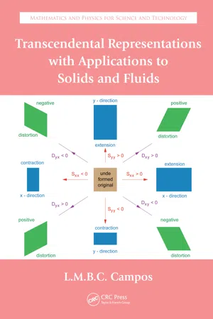

  Sign up to read

  Learn more about book
• 

  eBook - PDF

  Transcendental Representations with Applications to Solids and Fluids

  • Luis Manuel Braga da Costa Campos(Author)
  • 2012(Publication Date)
  • CRC Press

    (Publisher)

  This result is an immediate consequence of the imaginary change of variable (Equations 5.6a and 5.6b). The same transformation shows that Equations 5.115 through 5.118 hold for hyperbolic instead of circular functions suppressing the alternating signs: 347 Circular and Hyperbolic Functions sinh cosh sinh 2 2 1 2 0 1 2 2 1 Nz z N n n n N N n ( ) = --      = ---∑ 2 2 1 2 2 8 3 1 N n z N z N N --= + -( ) uni00A0 sinh ! sinh ! sinh 3 2 2 5 32 5 1 4 z N N N z + -( ) -( ) +  + + ( ) -( ) -( ) + + + + 2 2 1 1 2 2 1 2 2 2 2 1 m m m N N N m z ! sinh   2 1 2 1 N N z --sinh , (5.119) cosh cosh sinh 2 1 2 2 0 2 2 N z z N n n n N N n + ( )     = -      = -∑ 2 2 2 2 2 1 4 2 1 16 4 2 1 N n z N N z N N N -= + + ( ) + + ( ) -( ) uni00A0 ! sinh ! sin h uni00A0 ! ( ) 4 2 2 2 2 2 2 2 4 2 1 z m N N m N N N m m + + ( ) + -( ) -( ) --( )       + + sinh uni00A0 sinh , 2 2 2 2 m N N z z  (5.120) cosh ! sinh 2 2 1 2 2 1 2 2 2 2 2 Nz N n N n N n z N n N n ( ) = --( ) -+ ( ) -- n N N z N N = ∑ = + + 0 2 2 2 2 1 4 2 16 4 ! sinh ! -( ) + + ( ) -( 1 2 2 1 4 2 2 2 sinh ! z m N N m  ) --( )     + +   N m z z m N N 2 2 2 2 2 1 2 sinh sinh , (5.121) sinh ! 2 1 2 1 2 2 2 2 2 0 2 N z N n N n N n n N N + ( )     = + -( ) -+ ( ) = -∑  2 2 2 1 3 2 1 4 3 1 16 n N n z N z N N z sinh uni00A0 sinh ! ( ) sinh -+ = + ( ) + + + 5 2 1 2 2 1 2 5 2 2 ! sinh uni00A0 ! ( ) N N N z m N N m N m + ( ) -( ) +    + + ( ) + - 1 4 1 2 2 2 2 2 1 2 2 1 ( ) -( ) --( )     + + + + N N m z m N N   sinh sinh z      . (5.122) The hyperbolic sine/cosine of even (odd) multiples of the variable are given by Equations 5.119/5.121 (Equations 5.120/5.122) as a sum of powers of the hyperbolic sine of the variable.

  Sign up to read

  Learn more about book
• 

  eBook - PDF

  Calculus: Concepts and Methods

  • Ken Binmore, Joan Davies(Authors)
  • 2002(Publication Date)
  • Cambridge University Press

    (Publisher)

  258 7.6. Exercises The given equation therefore becomes 1 u 2 ∂ 2 z ∂ u 2 − 1 u 3 ∂ z ∂ u = 1 v 2 ∂ 2 z ∂v 2 − 1 v 3 ∂ z ∂v 7.6 Exercises 1. * ♣ Sketch the graphs of the functions defined by sinh x = 1 2 ( e x − e − x ) and cosh x = 1 2 ( e x + e − x ) . Prove that (i) d d x ( sinh x ) = cosh x (ii) d d x ( cosh x ) = sinh x . 2. * ♣ Explain why the equation y = sinh x always has a unique solution for x in terms of y . We write x = sinh − 1 y if and only if y = sinh x . Prove that cosh 2 x − sin 2 x = 1 and hence establish the formula d d y ( sinh − 1 y ) = 1 1 + y 2 . It is not possible to argue in a similar way from the equation y = cosh x . Explain why not. 3. ♣ Sketch the graph of the function defined by y = tanh x = sinh x cosh x Calculate the derivative of this function and explain how tanh − 1 y is defined for − 1 < y < 1. Prove that d d y ( tanh − 1 y ) = 1 1 − y 2 ( − 1 < y < 1 ) 4. * ♣ Differentiate ln ( y + y 2 + 1 ) and discuss the relevance of your result to Exercise 2. 5. ♣ Differentiate 1 2 ln[ ( 1 + y )/( 1 − y ) ] and discuss the relevance of your result to Exercise 3. 6. * Find a formula for a local inverse to the function f : R → R defined by y = f ( x ) = sin x at each of the points (i) x = π/ 6 (ii) x = 5 π/ 6 = π − (π/ 6 ) (iii) x = − 7 π/ 6 = − π − (π/ 6 ) Calculate the derivative of each local inverse directly from each formula. Evaluate these derivatives at the point y = 1 2 . Verify in each case that d x d y = d y d x − 1 . Explain why no local inverse exists at the point x = π/ 2. 259 Chapter 7. Inverse functions 7. The function f : R 2 → R 2 is defined by u v = f ( x , y ) = xy f ( x , y ) where f ( x , y ) = (i) y (ii) y + 2 x and (iii) x 2 + y 2 . In each of the three cases find the critical points of the function f . Then sketch the contours of each component function. Superimpose the contours and verify that the contours touch at critical points.

  Sign up to read

  Learn more about book