![]()
Chapter 1
Basic Concepts in Mathematical Finance
In this chapter, we give an overview of basic concepts in mathematical finance theory, and then explain those concepts in very simple cases, namely in the single-term finite market.
1.1 Price Processes
Price processes of financial assets are usually modeled as stochastic processes. So mathematical finance theory is based on probability theory, particularly on the theory of stochastic processes.
The price process of an underlying asset is generally denoted by St in this book. The process St is usually assumed to be positive and is expressed in the following form
The time parameter t usually runs in [0, T], T > 0, or [0, ∞), and sometimes we consider the discrete time case (t = 0, 1, . . . , T).
1.2 No-arbitrage and Martingale Measures
In mathematical finance theory, properties of the market where the financial assets are traded are vitally important. If the market works well, then the economy should work well, but if the market does not work well, then the economy shouldn't work.
An important property of the market is its efficiency. This is the “no-arbitrage” or “no free lunch” assumption in mathematical finance theory. A brief definition of arbitrage is: “an arbitrage opportunity is the possibility to make a profit in a financial market without risk and without net investment of capital” (see Delbaen and Schachermayer [30] p.4). The no-arbitrage assumption means that a market does not allow any arbitrage opportunity. The theory which is constructed on the no-arbitrage assumption is called “arbitrage theory”. In arbitrage theory, the martingale measure plays an essential role.
1.3 Complete and Incomplete Markets
If the market has enough commodities, then a new commodity should be a replica of old ones, and we don't need other new commodities. This concept of sufficient commodities in the market is the meaning of completeness in the market.
1.4 Fundamental Theorems
The two concepts introduced above are characterized by the concept of the martingale measure. The following two theorems are well known. (See Delbaen and Schachermayer (2006) [30] or Bjçork (2004) [9] for details.)
Theorem 1.1. (First Fundamental Theorem in Mathematical Finance). A necessary and sufficient condition for the absence of arbitrage opportunities is the existence of the martingale measure of the underlying asset process.
Theorem 1.2. (Second Fundamental Theorem in Mathematical Finance). Assume the absence of arbitrage opportunities. Then a necessary and sufficient condition for the completeness of the market is the uniqueness of the martingale measure.
If the market is arbitrage-free and complete, then the price of a contingent claim B, ° (B), is determined by
where Q is the unique martingale measure and r is the interest rate of the bond. In the case where the market satisfies the no-arbitrage assumption but does not satisfy the completeness assumption, then the price °(B) is supposed to be in the following interval:
where M is the set of all equivalent martingale measures. (See Theorem 2.4.1 in Delbaen and Schachermayer [30].)
1.5 The Black Scholes Model
The most popular and fundamental model in mathematical finance is the Black-Scholes model (geometric Brownian motion model). The explicit form of the underlying asset process of this model is given by
or equivalently in the stochastic differential equation (SDE) form
where µ is a real number, σ is a positive real number, and Wt is a Wiener process (standard Brownian motion).
The risk-neutral measure (= martingale measure)
Q is uniquely determined by Girsanov's theorem. Under
Q the process
is a Wiener process and the price process
St is expressed in the form
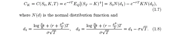
where r is the constant interest rate of a risk-free asset. The price of an option X is given by e−rT EQ [X]. The theoretical Black-Scholes price of the European call option, C (S0, K, T), with the strike price K and the fixed maturity T is given by the following formula:
1.6 Properties of the Black – Schol...