![]()
CHAPTER 1
Manifolds
1.1. Definition of a Manifold
A manifold, roughly, is a topological space in which some neighborhood of each point admits a coordinate system, consisting of real coordinate functions on the points of the neighborhood, which determine the position of points and the topology of that neighborhood; that is, the space is locally cartesian. Moreover, the passage from one coordinate system to another is smooth in the overlapping region, so that the meaning of “differentiable” curve, function, or map is consistent when referred to either system. A detailed definition will be given below.
The mathematical models for many physical systems have manifolds as the basic objects of study, upon which further structure may be defined to obtain whatever system is in question. The concept generalizes and includes the special cases of the Cartesian line, plane, space, and the surfaces which are studied in advanced calculus. The theory of these spaces which generalizes to manifolds includes the ideas of differentiable functions, .smooth curves, tangent vectors, and vector fields. However, the notions of distance between points and straight lines (or shortest paths) are not part of the idea of a manifold but arise as consequences of additional structure, which may or may not be assumed and in any case is not unique.
A manifold has a dimension. As a model for a physical system this is the number of degrees of freedom. We limit ourselves to the study of finite-dimensional manifolds.
Some preliminary definitions will facilitate the definition of a manifold. If X is a topological space, a chart at p ∈ X is a function μ : U → Rd, where U is an open set containing p and μ is a homeomorphism onto an open subset of Rd. The dimension of the chart μ: U → Rd is d . The coordinate functions of the chart are the real−valued functions on U given by the entries of values of μ; that is, they are the functions xi = ui ∘ μ: U → R, where ui: Rd → R are the standard coordinates on Rd. [The ui are defined by ui (a1,…, ad) = ai. The superscripts are not powers, of course, but are merely the customary tensor indexing of coordinates. If powers are needed, extra parentheses may be used, (x)3 instead of x3 for the cube of x , but usually the context will contain enough distinction to make such parentheses unnecessary.] Thus for each q ∈U, µq = (x1q ,…,xdq ), so we shall also write μ = (x1,…, xd). In other terminology we call uuu a coordinate map, U the coordinate neighborhood, and the collection (x 1,.., xd) coordinates or a coordinate system at p .
We shall restrict the symbols “ui” to this usage as standard coordinates on Rd. For R2 and R3 we shall also use x, y, z as coordinates as is customary, except that we shall usually treat them as functions.
A real-valued function f : V → R is C∞ (continuous to order ∞) if V is an open set in Rd and f has continuous partial derivatives of all orders and types (mixed and not). A function φ: V → Re is a C∞ map if the components ui ∘ φ: V → R are C∞, i = 1, …,e.
More generally ∈ is Ck, k a nonnegative integer, if all partial derivatives up to and including those of order k exist and are continuous. (C° means merely continuous.) A map φ is analytic if ui ∘ φ are real-analytic, that is, may be expressed in a neighborhood of each point by means of a convergent power series in cartesian coordinates having their origin at the point. Analytic maps are C∞ but not conversely.
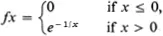
Problem 1.1.1. (a) Define f : R → R by
Show that f is C∞ and that all the derivatives of f at 0 vanish; that is, f(k)0 = 0 for every k.
(b) If g : R → R is analytic in a neighborhood of 0, then...