T-distribution

10 Key excerpts on "T-distribution"

• 

  No longer available |Learn more

  Handbook of Probability Distributions

  • (Author)
  • 2014(Publication Date)
  • Orange Apple

    (Publisher)

  This makes it useful for understanding the statistical behavior of certain types of ratios of random quantities, in which variation in the denominator is amplified and may produce outlying values when the denominator of the ratio falls close to zero. The Student's T-distribution is a special case of the generalised hyperbolic distribution. Introduction History and etymology In statistics, the T-distribution was first derived as a posterior distribution by Helmert and Lüroth. In the English literature, a derivation of the t -distribution was published in 1908 by William Sealy Gosset while he worked at the Guinness Brewery in Dublin. Since Gosset's employer forbade members of its staff from publishing scientific papers, his work was published under the pseudonym Student . The t -test and the associated theory became well-known through the work of R.A. Fisher, who called the distribution Student's distribution. Examples For examples of the use of this distribution. Characterization Student's T-distribution is the probability distribution of the ratio ________________________ WORLD TECHNOLOGIES ________________________ where • Z is normally distributed with expected value 0 and variance 1; • V has a chi-square distribution with ν (nu) degrees of freedom; • Z and V are independent. While, for any given constant μ , is a random variable of noncentral T-distribution with noncentrality parameter μ . Probability density function Student's T-distribution has the probability density function where ν is the number of degrees of freedom and Γ is the Gamma function. For ν even, For ν odd, The overall shape of the probability density function of the t -distribution resembles the bell shape of a normally distributed variable with mean 0 and variance 1, except that it is a bit lower and wider. As the number of degrees of freedom grows, the t -distribution approaches the normal distribution with mean 0 and variance 1.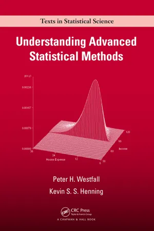

  Sign up to read

  Learn more about book
• 

  eBook - PDF

  Understanding Advanced Statistical Methods

  • Peter Westfall, Kevin S. S. Henning(Authors)
  • 2013(Publication Date)
  • Chapman and Hall/CRC

    (Publisher)

  In shorthand, T ∼ T m . 423 Chi-Squared, Student’s t , and F -Distributions, with Applications The derivation of the mathematical form of Student’s t -distribution is beyond the scope of this book, but the mathematical form itself is not so complex: Its kernel is given by p ( t ) ∝ (1 + t 2 / m ) −( m +1)/2 . Most statistical software packages have Student’s t -distribution, and include the appropriate constant of proportionality that makes the area under p ( t ) equal to 1.0. Figure 16.5 shows you how the t -distributions look for m = 1, 2, 10, and ∞; the case m = ∞ gives the standard normal distribution. Compared to the standard normal distribution, the t -distribution has the same median (0.0) but with variance df /( df − 2), which is larger than the standard normal’s variance of 1.0. The variance is infinite when df ≤ 2. The connection of the t -distribution to real-world data is as follows. Main Result for Student’s t -Distribution Suppose Y 1 , Y 2 , …, Y n ∼ iid N( m , s 2 ), and define T Y n = -( ) ( / ) m s ˆ . Then T ∼ T n − 1 . This result, along with Figure 16.5, explains why only 69.3% of the t -statistics were within the 0 ± 1.96 range in Example 16.1. Under the curve with df = 1 (the one with the shortest peak), only 69.3% of the area is between 0 ± 1.96. Using the T 1 cumulative distribution function rather than simulation, you can find this probability to be precisely Pr(−1.96 ≤ T 1 ≤ 1.96) = Pr( T 1 ≤ 1.96) − Pr( T 1 ≤ −1.96) = 0.84983 − 0.15017 = 0.6996. On the other hand, there is precisely 95% of the area under the standard normal curve (the solid curve) between 0 ± 1.96. It is mostly simple algebra to connect the main result with the definition of the t -distribution involving standard normals and chi-squares. But one result that requires higher math is this: If Y 1 , Y 2 , …, Y n ∼ iid N( m , s 2 ), then Y − and ˆ s are independent random variables.

  Sign up to read

  Learn more about book
• 

  eBook - ePub

  New Statistical Procedures for the Social Sciences

  Modern Solutions To Basic Problems

  • Rand R. Wilcox(Author)
  • 2013(Publication Date)
  • Psychology Press

    (Publisher)

  o )/s, and it is called Student's t distribution. (Gossett published his results under the name “Student.”) As will be seen, Student's t distribution plays an important role in many statistical procedures.

  Theorem 6.2.1 . If X1 , …, Xn is a random sample from a normal distribution, and if and s2 are the resulting sample mean and sample variance, then and s2 are independent random variables.

  The validity of Theorem 6.2.1 is far from obvious. Indeed you would expect it to be false since s2 =Σ(Xi - )2 /(n-1) which is an expression involving . In fact, in general, s2 and are dependent, but when normality is assumed they are independent.

  Definition 6.2.1 . Let Z be a standard normal random variable, and let Y be a chi-square random variable with v degrees of freedom where Z and Y are independene of one another. The distribution of

  is called a Student's t distribution with v degrees of freedom. (For convenience the subscript v will usually not be written.) The range of possible values of T is from ∞ to ∞. In addition, the distribution is symmetric about the origin, and its shape is very similar to the standard normal distribution. Percentage points of this distribution are given in Table A14. For instance, if v =10, Pr(T10 ≤1.812)=.95. Because the distribution is symmetric about the origin, Pr(T≤-t)-Pr(T≥t).

  If X1 , …, Xn is a random sample from a normal distribution, it has already been explained that ( n) ( -μ)/σ has a standard normal distribution, and (n-1)s2 /σ2 has a chi-square distribution with v =n-1 degrees of freedom. Also, these two quantities are independent of one another, and so

  has a Student's t distribution with v degrees of freedom. Note that the right side of (6.2.1a) is just n (

  Sign up to read

  Learn more about book
• 

  eBook - PDF

  Endocrine Manifestations of Systemic Autoimmune Diseases

  • Ronald Asherson(Author)
  • 2008(Publication Date)
  • Elsevier Science

    (Publisher)

  (This is why the t distribution is termed a small sample distribution.) More formally, the quantity T n = √ n(X n − µ) S 2 n has a t distribution with n − 1 degrees of freedom, where X n and S 2 n = ∑ n i=1 (X i −X n ) 2 (n−1) are, respectively, the mean and variance of a sample of size n taken from a normal distribution with mean µ and (known) standard devia- tion σ . Then the random variable T n → N (0, 1) as n → ∞. Stated alternatively, we may employ (9.20) to demonstrate that the t probability density function converges to the standard normal probability density function for large v or lim v→∞ f (t ; v) = 1 √ 2π e − 1 2 t 2 , −∞ < t < +∞. In this regard, since the asymptotic distribution of T = X−µ S/ √ n is N (0, 1), if a < b, then P(a < T < b) → 1 √ 2π b a e −t 2 /2 dt as n → ∞. 4. The mean and standard deviation of the t distribution are, respectively, E(T ) = 0, v > 1; (9.23) V (T ) = v v − 2 > 1, v > 2. (9.24) Given these restrictions on v, it follows that the t distribution does not have moments (about zero) of all orders; that is, if there are v degrees of freedom, then there are only v − 1 moments. Thus a t distribution has no mean when v = 1; it has no variance when v ≤ 2. In fact, all odd moments of T are zero. 5. The coefficient of skewness is α 3 = 0; (9.25) 360 Chapter 9 The Chi-Square, Student’s t, and Snedecor’s F Distributions and the coefficient of kurtosis is α 4 = 3 + 6 v − 4 , v ≥ 4 (9.26) with lim v→∞ α 4 = 3 (the value under normality). Selected quantiles of the t distribution appear in Table A.3 of the Appendix for various probabilities α (the area in the right-hand tail of the t distribution) and degrees of freedom values v. That is, the right-tailed quantile t α, v is the value of T for which P(T ≥ t α,v ) = +∞ t α,v f (t ; v) dt = α, 0 ≤ α ≤ 1 (9.26) (see Figure 9.5a). In this regard, we may view t α, v as an upper percentage point of the t distribution—the point for which the probability of a larger value of T is α.

  Sign up to read

  Learn more about book
• 

  eBook - PDF

  The Probability Handbook

  • Mary McShane-Vaughn(Author)
  • 2016(Publication Date)
  • ASQ Quality Press

    (Publisher)

  Examples of the use of Student’s t distribution include the following: • A quality manager uses Student’s t distribution to determine whether the mean burst strength of paper packages exceeds the minimum standard. • A Six Sigma Green Belt uses Student’s t distribution to test whether there is a difference in mean porosity for two different membrane designs. • A quality engineer uses a paired t test to evaluate the effectiveness of a new training program by analyzing the mean improvement in test scores before and after training. • A Six Sigma Black Belt uses Student’s t distribution to determine whether an independent variable in a regression model is a significant predictor of the response. Figure 5.36 Microsoft Excel function =t.test(). 118 Chapter Five 5.8 THE GAMMA DISTRIBUTION The gamma distribution is useful in modeling service times in queuing problems. It is a bit of a chameleon distribution, since in specific cases it becomes the expo- nential, chi-square, Rayleigh, and Erlang distributions, among others. 5.8.1 Probability Density Function The probability density function of the gamma distribution is shown in For- mula 5.29. Formula 5.29 Probability density of gamma distribution f(x) = , x > 0 Γ(α)β α x α–1 e –x/β As explained in Section 5.7.1, the term Г(α) is the gamma function. The gamma function is an integral, but for any positive integer n, the function simplifies to Г(n) = (n – 1)!. For example, Г(4) = (4 – 1)! = 6. Note also that = Γ √ 1 2 ) ) π . The gamma probability distribution function has two parameters, the shape parameter α and the scale parameter β. If α is an integer, then the cumulative dis- tribution function has the closed form shown in Formula 5.30. Formula 5.30 Cumulative distribution function of gamma distribution F(x) = 1 – e –x/β , x > 0 k! ( x/ β) k Σ k = 0 α – 1 Formulas 5.31 and 5.32 show the expected value and variance, respectively, of the gamma distribution.

  Sign up to read

  Learn more about book
• 

  eBook - ePub

  Calculus and Statistics

  • Michael C. Gemignani(Author)
  • 2014(Publication Date)
  • Dover Publications

    (Publisher)

  t; n). Given that t is a variate with density function f(t; n) and the entire set of real numbers as admissible range, find the mean, mode, and median of t. Prove that the distribution of t is symmetric with respect to 0. Using Table 4 find the value of t asked for, and the values of b in (d) and (e).

  a)

  b)

  c)

  d) Find b such that P(–b ≤ t ≤ b) = 0.95 if t has density function f(t; 11).

  e) Find b such that P(0 ≤ t ≤ b) = 0.475, where the density function of t is f(t; 15).

  4 . Twelve randomly chosen tomatoes are weighed; it is found that the mean weight is 6 ounces with a variance of 9. Find the probability that the true mean weight of tomatoes lies between 5 and 7 ounces. Find b such that there is a 0.95 probability that the mean weight of tomatoes lies between 6 – b and 6 + b.

  5 . Twenty-five ball bearings are found to have an average radius of 5.001 inches with a variance of 0.0025. What is the probability that the mean radius is really less than 5? Compute this probability using both the t- and normal distributions. Compare your results.

  6 . A random sample of 10 elements from a certain population has a mean of 15 and a variance of 16.

  a) Find b such that there is a 0.95 probability that the population mean lies between 15 – b and 15 + b.

  b) Find the b asked for in (a), assuming that the sample contains 15 observations (and all other factors remain unaltered).

  c) Find the b asked for in (a), assuming that the sample contains 20 observations. As the number of elements in the sample increases, what happens to b ?

  10.3 MORE ABOUT THE t-DISTRIBUTION

  The t-distribution can also be used in testing whether or not two populations have the same mean, provided certain conditions are satisfied and the samples are small enough to warrant the use of the t

  Sign up to read

  Learn more about book
• 

  eBook - PDF

  Statistics

  Unlocking the Power of Data

  • Robin H. Lock, Patti Frazer Lock, Kari Lock Morgan, Eric F. Lock, Dennis F. Lock(Authors)
  • 2016(Publication Date)
  • Wiley

    (Publisher)

  From now on, though, we will use the slightly more accurate T-distribution with n − 1 df, rather than the standard normal, when doing inference for a population mean based on a sample mean x and sample standard deviation, s. Fortunately, when using technology to find endpoints or probabilities for a T-distribution, the process is usually very similar to what we have already seen for the normal distribution. For larger samples, the results will be very close to what we get from a standard normal, but we will still use the T-distribution for consistency. For smaller samples, the T-distribution gives an extra measure of safety when using the sample standard deviation s in place of the population standard deviation . Conditions for the T-distribution For small samples, the use of the T-distribution requires that the population distri- bution be approximately normal. If the sample size is small, we need to check that the data are relatively symmetric and have no huge outliers that might indicate a departure from normality in the population. We don’t insist on perfect symmetry or an exact bell-shape in the data in order to use the T-distribution. The normality con- dition is most critical for small sample sizes, since for larger sample sizes the CLT for means kicks in. Unfortunately, it is more difficult to judge whether a sample looks “normal” when the sample size is small. In practice, we avoid using the T-distribution if the sample is small (say less than 20) and the data contain clear outliers or skew- ness. For more moderate sized samples (20 to 50) we worry if there are very extreme outliers or heavy skewness. When in doubt, we can always go back to the ideas of Chapters 3 and 4 and directly simulate a bootstrap or randomization distribution. If the sample size is small and the data are heavily skewed or contain extreme outliers, the T-distribution should not be used. Example 6.11 Dotplots of three different samples are shown in Figure 6.4.

  Sign up to read

  Learn more about book
• 

  eBook - PDF

  Statistics All-in-One For Dummies

  • Deborah J. Rumsey(Author)
  • 2022(Publication Date)
  • For Dummies

    (Publisher)

  By studying the behavior of all pos- sible samples, you can gauge where your sample results fall and understand what it means when your sample results fall outside of certain expectations. Chapter 12 IN THIS CHAPTER » Understanding the concept of a sampling distribution » Putting the Central Limit Theorem to work » Determining the factors that affect precision 264 UNIT 3 Distributions and the Central Limit Theorem Defining a Sampling Distribution A random variable is a characteristic of interest that takes on certain values in a random man- ner. For example, the number of red lights you hit on the way to work or school is a random variable; the number of children a randomly selected family has is a random variable. You use capital letters such as X or Y to denote random variables, and you use lowercase letters such as x or y to denote actual outcomes of random variables. A distribution is a listing, graph, or function of all possible outcomes of a random variable (such as X) and how often each actual outcome (x), or set of outcomes, occurs. (See Chapter 9 for more details on random variables and distributions.) For example, suppose a million of your closest friends each roll a single die and you record each actual outcome (x). A table or graph of all these possible outcomes (one through six) and how often they occurred represents the distribution of the random variable X. A graph of the distri- bution of X in this case is shown in Figure 12-1a. It shows the numbers 1 through 6 appearing with equal frequency (each one occurring 1 6 of the time), which is what you expect over many rolls if the die is fair. Now suppose each of your friends rolls this single die 50 times ( ) n 50 and you record the average, x . The graph of all their averages of all their samples represents the distribution of the random variable X . Because this distribution is based on sample averages rather than indi- vidual outcomes, this distribution has a special name.

  Sign up to read

  Learn more about book
• 

  eBook - PDF

  An Introduction to Uncertainty in Measurement

  Using the GUM (Guide to the Expression of Uncertainty in Measurement)

  • L. Kirkup, R. B. Frenkel(Authors)
  • 2006(Publication Date)
  • Cambridge University Press

    (Publisher)

  For very large ν and X % = 95 % , t X % ,ν = 1 . 96. Conventionally, in deriving the mathematical formula for the t -distribution, µ is regarded as the fixed population parameter, and ¯ x and s as the variables that vary with the particular sample. The probability density, p ( t , ν ), of the t -distribution for ν degrees of freedom is given by 13 p ( t , ν ) = K ( ν ) 1 + t 2 ν − ( ν + 1) / 2 , (10.6) where K ( ν ) ensures that the area under the probability density curve is unity. 14 In equation (10.4), t ν may be regarded as the difference between ¯ x and µ ex-pressed in terms of the number of standard deviations of the mean, s / √ n . We note that t ν is a dimensionless number . Figure 10.4 shows the probability density of the t -distribution for numbers of degrees of freedom ν = 3, 8, 20 and ∞ . The t -distribution is symmetric, even 13 See Kendall and Stuart (1969). 14 It may be shown that K ( ν ) = { ( ν + 1) / 2 } ( ν/ 2) 1 /πν, where denotes the gamma function. 10.2 The coverage interval using a T-distribution 171 Table 10.1. t values for ν degrees of freedom at the 95 % level of confidence ν t 95 % ,ν 3 3 . 18 8 2 . 31 20 2 . 09 ∞ 1 . 96 though it is the ratio of a Gaussian and therefore symmetrical distribution (the distribution of ¯ x − µ ) to an asymmetrical distribution (the distribution of s / √ n , as in figure 10.3(d)). For infinite ν , the t -distribution coincides exactly with the Gaussian distribution with mean zero and standard deviation 1. Figure 10.4 also shows the respective limits of the intervals along the horizontal axis which enclose 95 % of the total area. For the Gaussian case ( ν infinite), the limits are ± 1 . 96. As ν decreases, the peak of the t -distribution is reduced and more of the area under the probability density curve is located in the tails. 15 As a consequence, as ν decreases, 95 % of the total area is delimited by points further from the origin (which is at the centre of the horizontal axis).

  Sign up to read

  Learn more about book
• 

  eBook - ePub

  Introduction to Statistics for Forensic Scientists

  • David Lucy(Author)
  • 2013(Publication Date)
  • Wiley

    (Publisher)

  4 The normal distribution In Section 3.2 we saw how the binomial distribution could be used to calculate probabilities for specific outcomes for runs of events based upon either a known probability, or an observed probability, for a single event. We also saw how an empirical probability distribution can be treated in exactly the same way as a modelled distribution. Both these distributions were for discrete data types, or for continuous types made into discrete data. In this section we deal with the normal distribution, which is a probability distribution applied to continuous data. 4.1 The normal distribution The normal distribution † is possibly the most commonly used continuous distribution in statistical science. This is because it is a theoretically appealing model to explain many forms of natural continuous variation. Many of the discrete distributions may be approximated by the normal distribution for large samples. Most continuous variables, particularly from biological sciences, are distributed normally, or can be transformed to a normal distribution. Imagine a continuous random variable such as the length of the femur in adult humans. The mean length of this bone is about 400 mm, some are 450 mm and some are 350 mm, but there are not many in either of these categories. If the distribution is plotted then we expect to see a shape with its maximum height at about 400 mm tailing off to either side. These shapes have been plotted for both the adult human femur and adult human tibia in Figure 4.1. The tibia in any individual is usually shorter than the femur, however, Figure 4.1 tells us that some people have tibias which are longer than other people’s femurs. Notice how the mean of tibia measurements is shorter than the mean of the femur measurements

  Sign up to read

  Learn more about book