Physics
Vector Operations
Vector operations in physics involve mathematical operations such as addition, subtraction, and scalar multiplication performed on vectors. These operations are used to analyze and describe physical quantities that have both magnitude and direction, such as force and velocity. By manipulating vectors through these operations, physicists can solve problems related to motion, forces, and other physical phenomena.
Written by Perlego with AI-assistance
Related key terms
1 of 5
11 Key excerpts on "Vector Operations"
 eBook - PDF
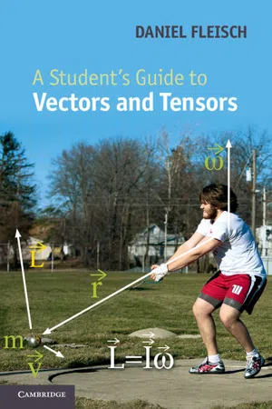
- Daniel A. Fleisch(Author)
- 2011(Publication Date)
- Cambridge University Press(Publisher)
2 Vector Operations If you were tracking the main ideas of Chapter 1 , you should realize that vectors are representations of physical quantities – they’re mathematical tools that help you visualize and describe a physical situation. In this chapter, you can read about a variety of ways to use those tools to solve problems. You’ve already seen how to add vectors and how to multiply vectors by a scalar (and why such operations are useful); this chapter contains many other “vector oper-ations” through which you can combine and manipulate vectors. Some of these operations are simple and some are more complex, but each will prove useful in solving problems in physics and engineering. The first section of this chapter explains the simplest form of vector multiplication: the scalar product. 2.1 Scalar product Why is it worth your time to understand the form of vector multiplication called the scalar or “dot” product? For one thing, forming the dot product between two vectors is very useful when you’re trying to find the projection of one vector onto another. And why might you want to do that? Well, you may be interested in knowing how much work is done by a force acting on an object. The first instinct of many students is to think of work as “force times distance” (which is a reasonable starting point). But if you’ve ever taken a course that went a bit deeper than the introductory level, you may remember that the definition of work as force times distance applies only to the special case in which the force points in exactly the same direction as the displacement of the object. In the more general case in which the force acts at some angle to the direction of the displacement, you have to find the component of the force along the displacement. That’s one example of exactly what the dot product can do for you, and you’ll find more in the problems at the end of this chapter. 25 eBook - PDF
- Bhag Singh Guru, Hüseyin R. Hiziroglu(Authors)
- 2009(Publication Date)
- Cambridge University Press(Publisher)
Force, velocity, torque, electric field, and acceleration are vector quantities. 14 15 2.3 Vector Operations A vector quantity is graphically depicted by a line segment equal to its magnitude according to a convenient scale, and the direction is indicated by means of an arrow, as shown in Figure 2.1a. We will represent a vector by placing an arrow over the letter. Thus, in Figure 2.1a, R represents a vector directed from point O toward point P. Figure 2.1b shows a few parallel vectors having the same length and direction ; they all represent the same vector. Two vectors A and B are equal ; i.e., A = B , if they have the same magnitude (length) and direction. We can only compare vectors if they have the same physical or geometrical meaning and hence the same dimensions. A vector of magnitude zero is called a null vector or a zero vector . This is the only vector that cannot be represented as an arrow because it has zero magnitude (length). A vector of unit magnitude (length) is called a unit vector . We can always represent a vector in terms of its unit vector. For example, vector A can be written as A = A a A (2.1) where A is the magnitude of A and a A is the unit vector in the same direction of A such that a A = A A (2.2) Figure 2.1 2.3 Vector Operations ................................. Adding, subtracting, multiplying, and/or dividing scalar quantities is second nature to most of us. For example, if we want to add two scalars having the same units, we just add their magnitudes. The process of addition in terms of vectors is not this simple, nor are subtraction and multiplication of two vectors. Note that vector division is not defined. 2.3.1 Vector addition To add two vectors A and B we draw two representative vectors A and B in such a way that the initial point (tail) of B coincides with the final 16 2 Vector analysis point (tip) of A , as illustrated by the solid lines in Figure 2.2.
- K. F. Riley, M. P. Hobson(Authors)
- 2011(Publication Date)
- Cambridge University Press(Publisher)
9 Vector algebra This chapter introduces space vectors and their manipulation. Firstly we deal with the description and algebra of vectors, then we consider how vectors may be used to describe lines, planes and spheres, and finally we look at the practical use of vectors in finding distances. The calculus of vectors will be developed in a later chapter; this chapter gives only some basic rules. 9.1 Scalars and vectors • • • • • • • • • • • • • • • • • • • • • • • • • • • • • • • • • • • • • • • • • • • • • • • • • • • • • • • • • • • • • • • • • The simplest kind of physical quantity is one that can be completely specified by its magnitude, a single number, together with the units in which it is measured. Such a quantity is called a scalar , and examples include temperature, time and density. A vector is a quantity that requires both a magnitude ( ≥ 0) and a direction in space to specify it completely; we may think of it as an arrow in space. A familiar example is force, which has a magnitude (strength) measured in newtons and a direction of application. The large number of vectors that are used to describe the physical world include velocity, displacement, momentum and electric field. Vectors can also be used to describe quantities such as angular momentum and surface elements (a surface element has a magnitude, defined by its area, and a direction defined by the normal to its tangent plane); in such cases their definitions may seem somewhat arbitrary (though in fact they are standard) and not as physically intuitive as for vectors such as force. A vector is denoted by bold type, the convention of this book, or by underlining, the latter being much used in handwritten work. This chapter considers basic vector algebra and illustrates just how powerful vector analysis can be. All the techniques are presented for three-dimensional space but most can be readily extended to more dimensions. eBook - PDF
Mathematical Methods for Physicists
A Concise Introduction
- Tai L. Chow(Author)
- 2000(Publication Date)
- Cambridge University Press(Publisher)
1 Vector and tensor analysis Vectors and scalars Vector methods have become standard tools for the physicists. In this chapter we discuss the properties of the vectors and vector fields that occur in classical physics. We will do so in a way, and in a notation, that leads to the formation of abstract linear vector spaces in Chapter 5. A physical quantity that is completely specified, in appropriate units, by a single number (called its magnitude) such as volume, mass, and temperature is called a scalar. Scalar quantities are treated as ordinary real numbers. They obey all the regular rules of algebraic addition, subtraction, multiplication, division, and so on. There are also physical quantities which require a magnitude and a direction for their complete specification. These are called vectors if their combination with each other is commutative (that is the order of addition may be changed without aecting the result). Thus not all quantities possessing magnitude and direction are vectors. Angular displacement, for example, may be characterised by magni-tude and direction but is not a vector, for the addition of two or more angular displacements is not, in general, commutative (Fig. 1.1). In print, we shall denote vectors by boldface letters (such as A ) and use ordin-ary italic letters (such as A ) for their magnitudes; in writing, vectors are usually represented by a letter with an arrow above it such as ~ A . A given vector A (or ~ A ) can be written as A A ^ A ; 1 : 1 where A is the magnitude of vector A and so it has unit and dimension, and ^ A is a dimensionless unit vector with a unity magnitude having the direction of A . Thus ^ A A = A . 1 A vector quantity may be represented graphically by an arrow-tipped line seg-ment. The length of the arrow represents the magnitude of the vector, and the direction of the arrow is that of the vector, as shown in Fig. eBook - PDF
Learning and Teaching Mathematics using Simulations
Plus 2000 Examples from Physics
- Dieter Röss(Author)
- 2011(Publication Date)
- De Gruyter(Publisher)
In quantum mechanics one works with vectors in the infinitely dimensional Hilbert space. Plane problems can be described by two-dimensional vectors that can be considered to lie in the complex plane. Vector algebra and vector analysis, in which partial differentiations take place, are an especially important mathematical tool of theoretical physics and therefore are often treated in depth in many textbooks for first year students.Their objects and oper-ations are not easily accessible to the untrained imagination. Therefore, the following sections concentrate only on the interactive visualization of fundamental aspects. 8.2 3D-visualization of vectors The classical visual presentation of a vector is an arrow in space, whose length defines an absolute value and whose orientation defines a direction. The place at which the arrow is situated is arbitrary; one can, for example, let it start as a zero-point vector from the origin of a Cartesian system of coordinates. Thus its endpoint (the tip of the arrow) is described by the three space coordinates x; y; z in this system of coordinates. Its length a , also referred to as the absolute value of the vector, is obtained from the theorem of Pythagoras as a D p x 2 C y 2 C z 2 . It obviously does not matter how the system of coordinates, with respect to which the coordinates of the vector are defined, is orientated in space. Under a change of the coordinate system (translation or rotation), the individual coordinates also change, but the position and length of the vector are not affected by this. They are invariant under translation and rotation. This property provides the definition of a vector. Quantities that can be characterized by specifying a single number for every point in space are called scalar , in contract to vectors; an example would be a density-or temperature distribution. The three-dimensional zero-point vector represents the position coordinates of a point in space.
- Henrik Aratyn, Constantin Rasinariu;;;(Authors)
- 2005(Publication Date)
- WSPC(Publisher)
Part I Mathematical Methods Vectors and Vector Calculus VECTORS on a plane or in three dimensional space can be thought of as arrows with magnitude and direction. One can view a collection of vectors satisfying a set of simple algebraic rules as a linear structure called vector space. This gives rise to a more abstract notion of a vector as an element of a vector space making it possible to include more abstract objects like functions and polynomials in the theory of vectors. For vector spaces we discuss topics like: linear dependence and independence, bases and dimension. In case of three dimensional vectors we learn how to project a vector on a given direction and how to construct orthogonal bases. In order to measure variations of forces and velocities and to evaluate magnetic fluxes we must learn how to differentiate and integrate three dimensional vectors. Vector calculus extends the notion of one-dimensional calculus and provides tech- niques for taking derivatives of multi-dimensional objects and dealing with line, surface and volume integrals. In this Chapter, we will learn the fundamental theo- rems of vector calculus and apply them to various coordinate systems. 1 .I Vectors and Vector Spaces 1.1.1 Vectors Scalar quantities like mass, temperature, charge or pressure are uniquely specified by their magnitude. Physics also requires vector quantities like velocity, force, angular momentum, which have magnitude as well as direction. The simplest vector quantity is displacement associated with change of position. Every displacement has an initial or starting point and a final point. Let us consider displacenients that have a conimon starting point: the origin. Any point in space can be understood as the final point of a displacement from the origin. We will depict such displacements by an arrow starting at the origin and ending at the final 2 Chapter 1 Vectors and Vector Calculus 3 + + point A or B. We will denote such displacements by vectors A or B. eBook - PDF
- Daniel Kleppner, Robert Kolenkow(Authors)
- 2013(Publication Date)
- Cambridge University Press(Publisher)
VECTORS AND KINEMATICS 1 1.1 Introduction 2 1.2 Vectors 2 1.2.1 Definition of a Vector 2 1.3 The Algebra of Vectors 3 1.3.1 Multiplying a Vector by a Scalar 3 1.3.2 Adding Vectors 3 1.3.3 Subtracting Vectors 3 1.3.4 Algebraic Properties of Vectors 4 1.4 Multiplying Vectors 4 1.4.1 Scalar Product (“Dot Product”) 4 1.4.2 Vector Product (“Cross Product”) 6 1.5 Components of a Vector 8 1.6 Base Vectors 11 1.7 The Position Vector r and Displacement 12 1.8 Velocity and Acceleration 14 1.8.1 Motion in One Dimension 14 1.8.2 Motion in Several Dimensions 15 1.9 Formal Solution of Kinematical Equations 19 1.10 More about the Time Derivative of a Vector 22 1.10.1 Rotating Vectors 23 1.11 Motion in Plane Polar Coordinates 26 1.11.1 Polar Coordinates 27 1.11.2 d ˆ r / dt and d ˆ θ / dt in Polar Coordinates 29 1.11.3 Velocity in Polar Coordinates 31 1.11.4 Acceleration in Polar Coordinates 34 Note 1.1 Approximation Methods 36 Note 1.2 The Taylor Series 37 Note 1.3 Series Expansions of Some Common Functions 38 Note 1.4 Di ff erentials 39 Note 1.5 Significant Figures and Experimental Uncertainty 40 Problems 41 2 VECTORS AND KINEMATICS 1.1 Introduction Mechanics is at the heart of physics; its concepts are essential for under-standing the world around us and phenomena on scales from atomic to cosmic. Concepts such as momentum, angular momentum, and energy play roles in practically every area of physics. The goal of this book is to help you acquire a deep understanding of the principles of mechanics. The reason we start by discussing vectors and kinematics rather than plunging into dynamics is that we want to use these tools freely in dis-cussing physical principles. Rather than interrupt the flow of discussion later, we are taking time now to ensure they are on hand when required. 1.2 Vectors The topic of vectors provides a natural introduction to the role of math-ematics in physics. By using vector notation, physical laws can often be written in compact and simple form. eBook - PDF
- David J. Griffiths(Author)
- 2017(Publication Date)
- Cambridge University Press(Publisher)
C H A P T E R 1 Vector Analysis 1.1 VECTOR ALGEBRA 1.1.1 Vector Operations If you walk 4 miles due north and then 3 miles due east (Fig. 1.1), you will have gone a total of 7 miles, but you’re not 7 miles from where you set out—you’re only 5. We need an arithmetic to describe quantities like this, which evidently do not add in the ordinary way. The reason they don’t, of course, is that displace- ments (straight line segments going from one point to another) have direction as well as magnitude (length), and it is essential to take both into account when you combine them. Such objects are called vectors: velocity, acceleration, force and momentum are other examples. By contrast, quantities that have magnitude but no direction are called scalars: examples include mass, charge, density, and temperature. I shall use boldface (A, B, and so on) for vectors and ordinary type for scalars. The magnitude of a vector A is written |A| or, more simply, A. In diagrams, vec- tors are denoted by arrows: the length of the arrow is proportional to the magni- tude of the vector, and the arrowhead indicates its direction. Minus A (−A) is a vector with the same magnitude as A but of opposite direction (Fig. 1.2). Note that vectors have magnitude and direction but not location: a displacement of 4 miles due north from Washington is represented by the same vector as a displacement 4 miles north from Baltimore (neglecting, of course, the curvature of the earth). On a diagram, therefore, you can slide the arrow around at will, as long as you don’t change its length or direction. We define four Vector Operations: addition and three kinds of multiplication. 3 mi 5 mi 4 mi FIGURE 1.1 −A A FIGURE 1.2 1 2 Chapter 1 Vector Analysis A A B B (A+B) (B+A) FIGURE 1.3 −B A (A−B) FIGURE 1.4 (i) Addition of two vectors. Place the tail of B at the head of A; the sum, A + B, is the vector from the tail of A to the head of B (Fig. 1.3). eBook - PDF
- Ronald Huston, C Q Liu(Authors)
- 2001(Publication Date)
- CRC Press(Publisher)
Chapter 2 VECTOR ANALYSIS AND PRELIMINARY CONSIDERATIONS 2.1 Introduction In this chapter we briefly review and present some operational formulas, primarily from elementary vector analysis, which form the basis for the dynamics formulations of the subsequent chapters. We develop and illustrate many of the formulas through a series of examples. The references at the end of this chapter provide a more comprehensive review. 2.2 Fundamental Concepts • Vectors — Mathematically, a vector is an element of a vector space [2.1, 2.2, 2.3]. Since dynamics is fundamentally a geometric subject it is helpful to think of vectors as being directed line segments. Symbolically, vectors are written in bold face type (for example, v). • Vector Characteristics — The characteristics of a vector are its magnitude (length) and direction (orientation and sense). The units of a vector are the same units of those of its magnitude. The magnitude of a vector, say v, is written as | v | . • Equality of Vectors — Two vectors a and b are said to be equal (a = b) if they have the same characteristics (magnitude and direction). • Scalar — A scalar is simply a variable or parameter. Scalars may be either real or complex numbers, although in dynamics they are generally real numbers. They may be positive or negative. Frequently appearing scalars in dynamics are time, distance, mass, and force, velocity and acceleration magnitudes. 12 Vector Analysis 13 • Multiplication of Scalars and Vectors — Let D be a scalar and let V be a vector. Then the product sV is a vector with the same orientation and sense as V if s is positive, and with the same orientation but opposite sense of V if s is negative. The magnitude of sV is |s| |V|. (See Section 2.5.) • Negative Vector — The negative of vector V, written as -V, is a vector with the same magnitude and orientation as V, but with opposite sense to that of V. eBook - PDF
- Jerry Ginsberg(Author)
- 2007(Publication Date)
- Cambridge University Press(Publisher)
Newton’s Laws pertain only to a particle. The derivation of a variety of principles that extend these laws to bodies having significant dimensions will be treated in depth. We will limit our attention to systems in which all bodies may be considered to be particles or rigid bodies. The dynamics of flexible bodies, which is the subject of vibrations, is founded on the kinematics and kinetics concepts we will estab-lish. We shall begin by reviewing the fundamental aspects of Newton’s Laws. Although the reader is likely to have already studied these concepts, the intent is to provide a consistent foundation for later developments. 1.1 Vector Operations 1.1.1 Algebra and Computations Almost every quantity of importance in dynamics is vectorial in nature. Such quantities have a direction in which they are oriented, as well as a magnitude. The kinematical 1 2 Basic Considerations vectors of primary importance for our initial studies are position, velocity, and accelera-tion, and the kinetics quantities are force and moment. Some quantities have magnitude and direction, but are not vectors. One example, which will play a major role in Chap-ter 3, is a finite rotation about an axis. An additional requirement for vector quantities is that they add according to the parallelogram law. This entails a graphical representation of vectors in which an arrow indicates the direction of the vector and the length of the arrow is proportional to the magnitude of the vector. A graphical representation of the summation operation is shown in Fig. 1.1 (a), which shows that the addition of two vec-tors ¯ A and ¯ B may be constructed in either of two ways. Vectors ¯ A and ¯ B may be placed tail to tail, and then considered to form two sides of a parallelogram. Then ¯ A + ¯ B is the main diagonal, with the sense defined to be from the common tail to the opposite corner. An alternative picture places the tail of ¯ B at the head of ¯ A . eBook - PDF
- Tom M. Apostol(Author)
- 2019(Publication Date)
- Wiley(Publisher)
W. Gibbs (1839–1903) and O. Heaviside (1850–1925), and a new subject called vector algebra sprang into being. It was soon realized that vectors are the ideal tools for the exposition and simplification of many important ideas in geometry and physics. In this chapter we propose to discuss the elements of vector algebra. Applications to analytic geometry are given in Chapter 13. In Chapter 14 vector algebra is combined with the methods of calculus, and applications are given to both geometry and mechanics. There are essentially three different ways to introduce vector algebra: geometrically, analyt- ically, and axiomatically. In the geometric approach, vectors are represented by directed line segments, or arrows. Algebraic operations on vectors, such as addition, subtraction, and multipli- cation by real numbers, are defined and studied by geometric methods. In the analytic approach, vectors and Vector Operations are described entirely in terms of num- bers, called components. Properties of the Vector Operations are then deduced from corresponding properties of numbers. The analytic description of vectors arises naturally from the geometric description as soon as a coordinate system is introduced. 445 446 Vector algebra In the axiomatic approach, no attempt is made to describe the nature of a vector or of the algebraic operations on vectors. Instead, vectors and Vector Operations are thought of as unde- fined concepts of which we know nothing except that they satisfy a certain set of axioms. Such an algebraic system, with appropriate axioms, is called a linear space or a linear vector space. Examples of linear spaces occur in all branches of mathematics, and we will study many of them in Chapter 15. The algebra of directed line segments and the algebra of vectors described by components are merely two examples of linear spaces.
Index pages curate the most relevant extracts from our library of academic textbooks. They’ve been created using an in-house natural language model (NLM), each adding context and meaning to key research topics.