The Calculus

A Genetic Approach

Otto Toeplitz

• Publisher: University of Chicago Press
• Year: 2018
• ISBN:
  9780226806693
• Topic: Matematica
• Subtopic: Matematica generale

When first published posthumously in 1963, this bookpresented a radically different approach to the teaching of calculus.In sharp contrast to the methods of his time, Otto Toeplitz did not teach calculus as a static system of techniques and facts to be memorized. Instead, he drew on his knowledge of the history of mathematics and presented calculus as an organic evolution of ideas beginning with the discoveries of Greek scholars, such as Archimedes, Pythagoras, and Euclid, and developing through the centuries in the work of Kepler, Galileo, Fermat, Newton, and Leibniz. Through this unique approach, Toeplitz summarized and elucidated the major mathematical advances that contributed to modern calculus.Reissued for the first time since 1981 and updated with a new foreword, this classic text in the field of mathematics is experiencing a resurgence of interest among students and educators of calculus today.

3

DIFFERENTIAL AND INTEGRAL CALCULUS

18. TANGENT PROBLEMS

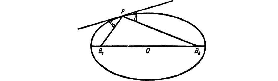
Tangent problems are easier than area problems. The Greeks knew very well how to construct a tangent at a point P of a circle (Fig. 63) by drawing the perpendicular to the radius OP. In the case of the ellipse, the construction of the tangent ab rested on the theorem that the tangent at P forms equal angles with the two focal radii drawn from P (Fig. 64). Similarly, in the case of the hyperbola.

FIG. 63

FIG. 64

(The Greeks, in fact, treated many tangent problems. Archimedes in his treatise on the spiral₂₉—the one which we still call the Spiral of Archimedes—deals with nothing else but the construction of the tangent and the calculation of the area of a sector of the spiral.)

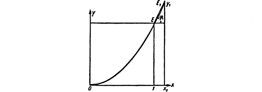
When in modern times—meaning the first half of the seventeenth century—Greek mathematics was resumed, numerous new tangent problems were treated. But, because a curve was now understood as a geometrical representation of a computational expression, the method of dealing with tangent problems was changed, and a new element entered into them. For instance, in the case of the parabola, which is the geometric representation of the function y = x², we find the tangent at the point E(1, 1) (Fig. 65). We take a value of x close to 1 and call it x₁; the corresponding value of the function is y₁ = x²₁. Let E₁ be the point (x₁, y₁); let φ₁ be the angle which the secant EE₁ makes with the horizontal through E; then we have

And here is the new method that we wanted to introduce by the example. We regard the tangent as the limiting position of the secant EE₁, which results when x₁ approaches 1 indefinitely.

So much for the principle. With simple mathematical manipulation, we find

FIG. 65

FIG. 66

If x₁ approaches 1, x₁ + 1 approaches 2; this means that if φ is the angle between the tangent and the x-axis

tan φ = 2.

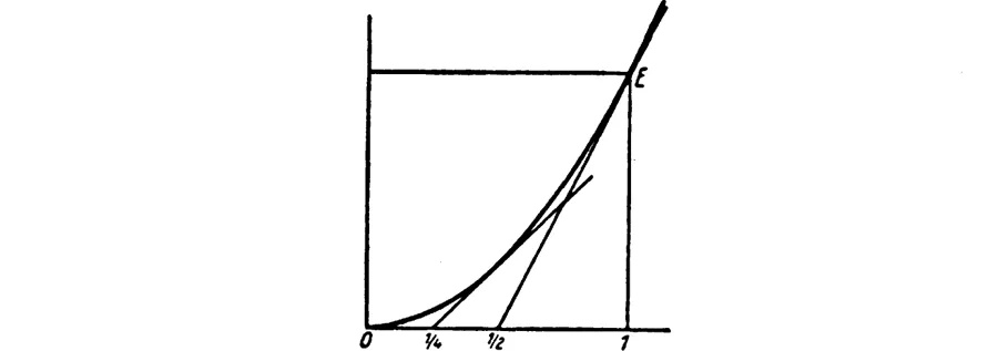
Thus, in the limit, the opposite side is exactly twice as long as the adjacent side. Hence we need not even draw the parabola to construct the tangent at E. We simply connect with E the midpoint of the segment with ends 0 and 1.

In the same way we find for any other x that, as x₁ → x,

So, for

we have tan φ = 1 which means that the tangent at

is constructed by connecting

with

. For drawing the parabola, the knowledge of these two tangents is more useful than the plotting of many of its points (Fig. 66).

In Section 12 we saw how Fermat determined

Since

for x → 1, this becomes n + 1. This same principle gives the general construction of the tangent at any point of the curve y = xⁿ. As x₁ → x,

Next we introduce a new symbol and a new terminology. Quite generally we shall write

and call the value f′(x) the “derivative” of f at x. It is equal to tan φ where φ is the inclination to the x-axis of the tangent (Fig. 67).

FIG. 67

For these “derivatives” we shall now obtain some very general results, which correspond to the two principles of Cavalieri (see above, Sec. 13).

1. Let y = f(x) + g(x).

Then we have

which leads to

2. Let y = ρf(x).

Then we have

which leads to

3. For more than two summands these two results give

4. Applying this to the case

and considering that

we obtain

This means that we can draw tangents at every point of any curve c₁x + c2x² + . . . +c_nxⁿ.

Fermat, whose achievements in the theory of areas we discussed previously, was a master also in tangent problems. He knew fully how to handle them in situations like those above, as well as for many other curves; therefore, he is often said to have known differential calculus.

19. INVERSE TANGENT PROBLEMS

In contrast with area problems, those concerning tangents presented no difficulties, no matter what curves were taken, until the problem was inverted; that is, the tangent was given and the curve had to...