What is the IS-LM Model?

Defining the IS-LM model 

The IS-LM model determines the equilibrium between interest rates and output in an economy. This model was developed during the Keynesian economics era by British economist John Hicks, who is considered one of the most influential economists of the twentieth century for his microeconomic and macroeconomic contributions. Indeed, in John Hicks: His Contributions to Economic Theory & Application (2018), O.F. Hamouda describes the importance of his findings: 

What Hicks accomplished was truly groundbreaking. He took Keynes’ The General Theory of Employment, Interest and Money (1936, [2021]), which was considered the “Bible” of economic thought at the time, and condensed it into graphical form to explain the relationship between output and interest rates in an economy. He did so by looking into the different component variables that make up the IS-LM model: investment, savings, liquidity and money supply.

Originally, Hicks described the IS-LM model as the “SI-LL” model in his paper “Mr. Keynes and the ‘Classics’; A Suggested Interpretation” (Hicks, 1937). It was Alvin Hansen, American economist and professor at Harvard University, who transformed the SI-LL into the IS-LM model, and popularized the theory in his book Fiscal Policy & Business Cycles (1941, [2013]). It is for this reason that this graphical and mathematical representation of Keynesian macroeconomic theory is often referred to as the Hicks-Hansen IS-LM model. 

The IS Curve

The IS-LM model is made up of two curves: the IS curve, and the LM curve. These curves are mapped in a graph, where the vertical y-axis represents the interest rate (r) and the horizontal x-axis the output or GDP (Y) in an economy (Figure 1). In the graph, the IS and LM curves represent a market in the economy. In this context, the word “market” does not refer to that of a product or service, but instead to a division or sector of the economy. For example, the money market concerns all monetary transactions in an economy. 

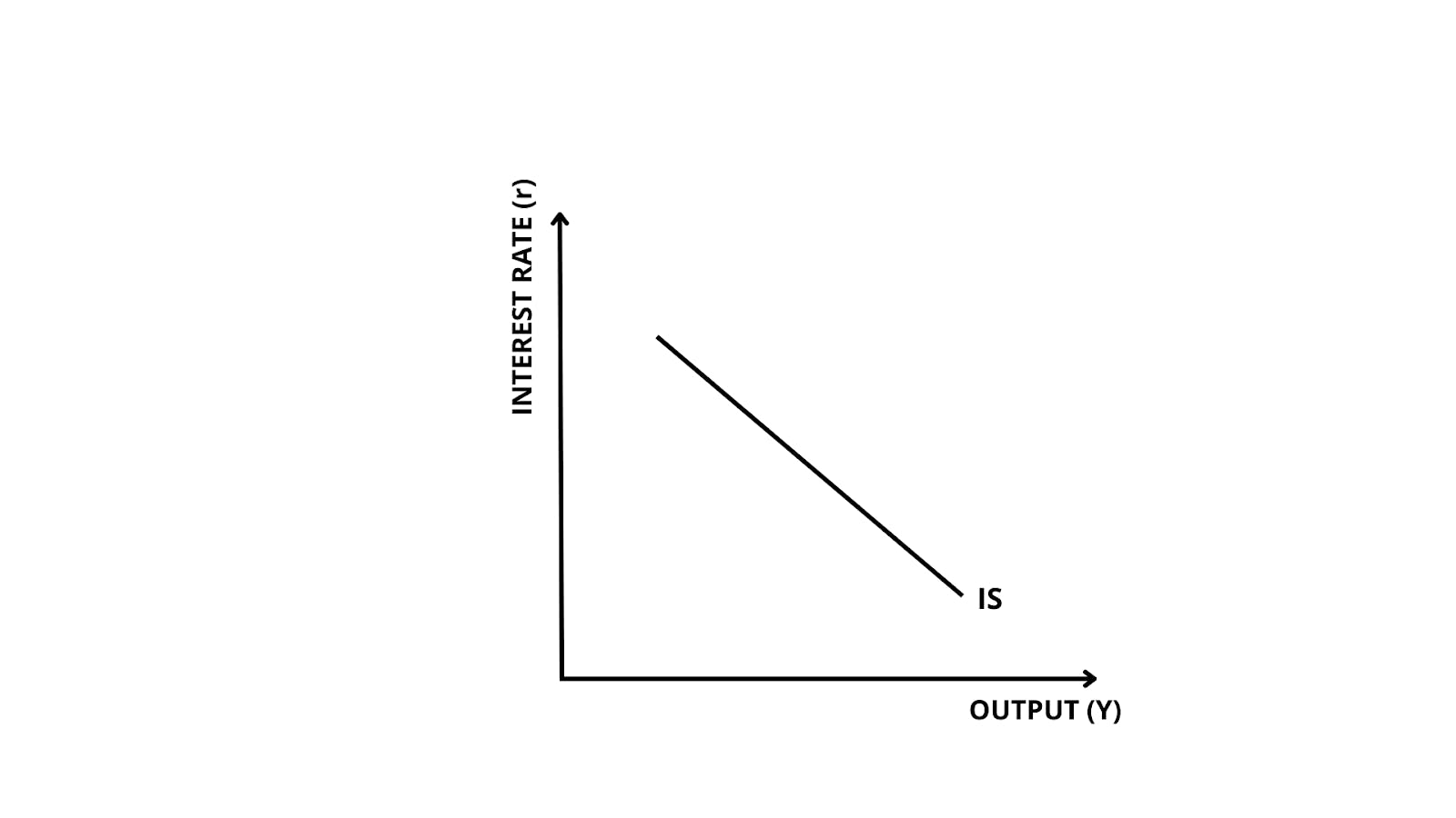
Figure 1 — IS Curve

As explained in the textbook Intermediate Macroeconomics (Robert J. Barro, Angus C. Chu, and Guido Cozzi, 2017) the IS curve stands for the investment-saving curve and represents the “goods market” where investment and savings are the main actors. 

The IS curve is downward sloping (Figure 1) because intuitively, at lower interest rates (i.e., the price of borrowing money), there is more demand for loans to finance investment. Savings decrease and investment increases. This translates to higher output in the goods market, which is directly proportional to investment (I).

The LM Curve

The LM curve explores the liquidity-money dynamic in the money market. When economists talk about liquidity, they are referring to the ease and speed with which assets such as bonds can be converted into cash (or into non-asset forms). Knowing this, people can choose to keep their assets in asset form, which rewards them with an interest payment, or they can choose to convert them into non-interest-earning forms such as cash or money. The LM curve represents this dynamic as an upward sloping curve (Figure 2), arguing that as output increases (Y), consumption and spending in economies rise (with more people wanting to have money in liquid, cash form). This, in turn, causes interest rates to rise to encourage people to transform their money back into assets and maintain the liquidity equilibrium in an economy. 

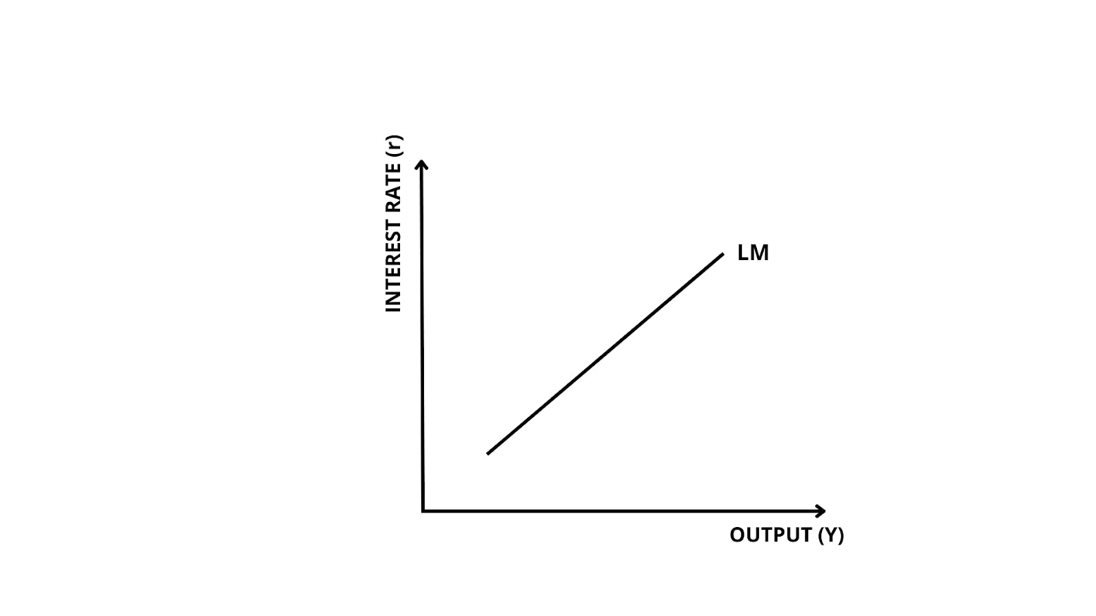
Figure 2 — LM Curve

This liquidity-money dynamic is often referred to as the “liquidity preference” theory; a term coined by Keynes himself, and explained here by Fernando J. Cardim de Carvalho:

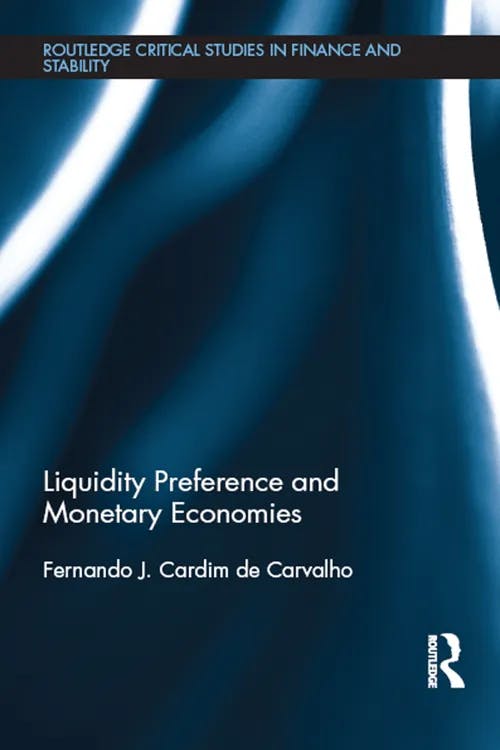
The IS-LM Curve — an example

It is now time to bring together the IS and LM curves with an example. Recall that the IS-LM model aims to find the equilibrium or optimal level of interest rate in an economy at a given output level. This equilibrium is found at the intersection of both curves, as shown in Figure 3. 

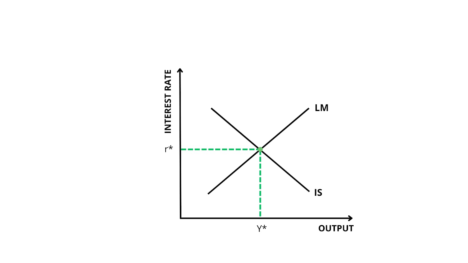
Figure 3 — Intersection of IS-LM Curve

In real life, the IS-LM model is used to understand the effects that changes in the goods or money markets (respectively represented by the IS and LM curves) will have on the output and general interest rate in an economy. For example, say that the government decides to increase spending in an economy. This is known as an expansionary fiscal policy. As explained above, because government spending is one of the components of the goods market (represented by the IS curve), an expansionary fiscal policy will shift the IS curve to the right; there is an increase in the economy’s consumption and output (Figure 4). At this point, it would be logical to think that the new equilibrium settles at a point where an economy has a higher output and general interest rate. 

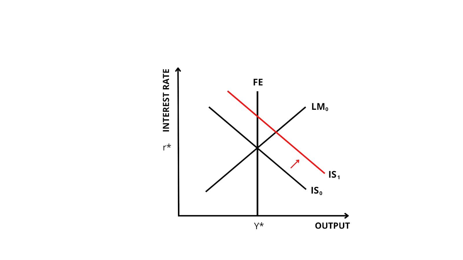
Figure 4 — FE Curve and Shift in IS Curve Due to Increased Government Spending

However, a third component of the graph comes in. The vertical full employment (FE) curve shown in Figure 2 represents the output an economy can produce with full employment in the long run. This is also known as the long-run aggregate supply curve (LRAS). Unless something increases the productive potential of an economy (e.g., an increase in the population), the FE curve will not move. This means that in the short term, the IS and LM curves will have to readjust to go back to the level of output dictated by the FE curve (Y*). 

In our example, where only government spending has increased (i.e., there is no change in the productive capacity of the nation), the LM curve will shift inwards (Figure 5) to bring the economy back to the initial output level (Y*). In other words, the LM curve contracts because the money supply (cash) available in the economy decreases, with more people using money to consume in response to increased government spending. Therefore, the new equilibrium (Figure 6) settles at a higher interest rate (r*1 ) and the same initial level of output (Y*). 

Figure 5 — Inward Shift of the LM Curve

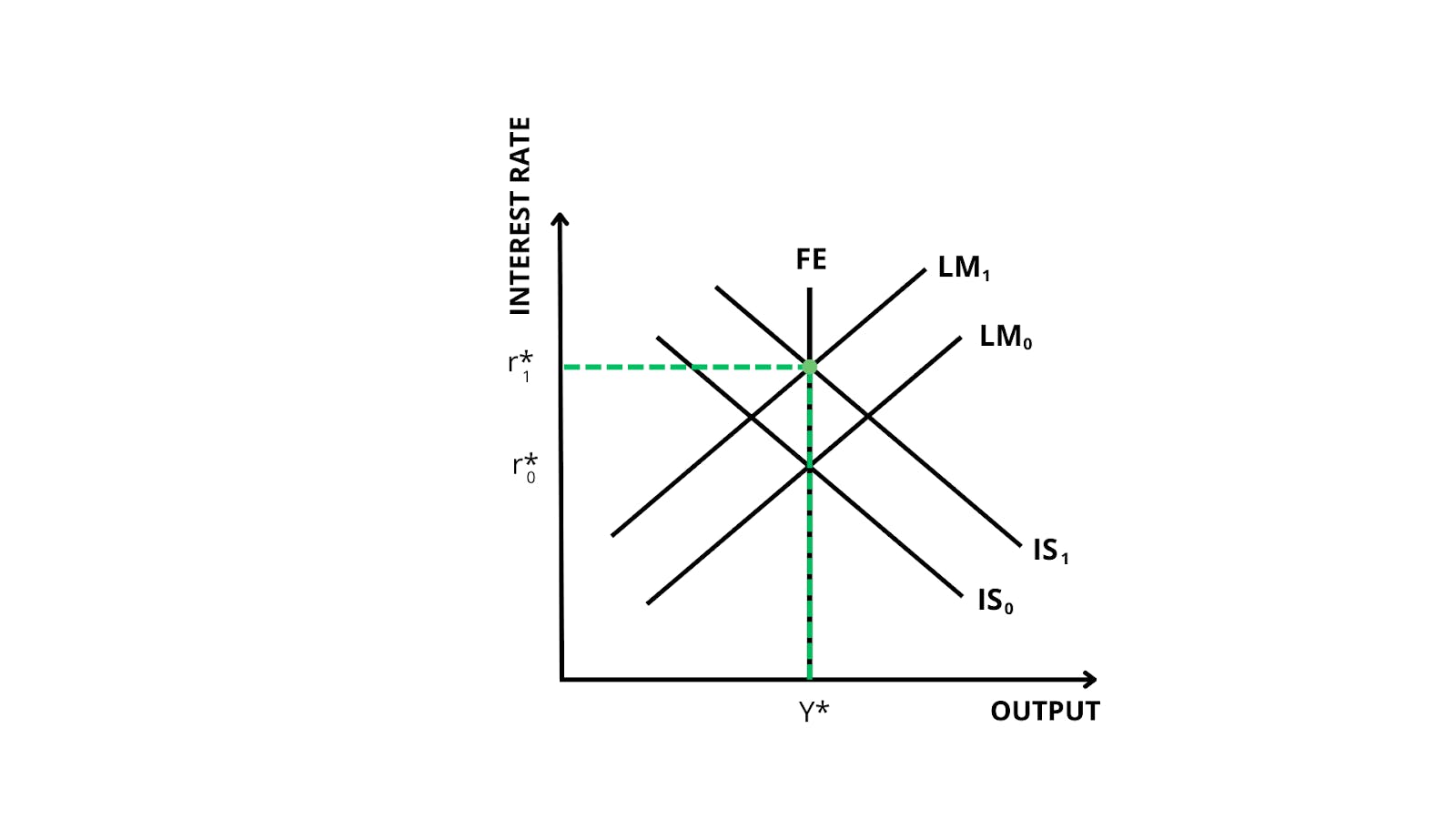
Figure 6 — New Equilibrium Output and Interest Rate After Increased Government Spending

There are many other examples and circumstances where the IS-LM model can be applied. For instance, there may be a situation where central banks opt for quantitative easing (i.e., increasing money supply in the economy). This would have an effect on the LM curve, not the IS curve. It may also be the case that the IS and LM curves remain untouched and there is a sudden increase in the LRAS of an economy (e.g., if there is an increase in the capital and machinery available for production). All these scenarios are thoroughly explained and graphically illustrated in Chapter 6 of the textbook Intermediate Macroeconomics (Barro, Chu, and Cozzi, 2017).

Limitations of the IS-LM model

Like every economic model, the IS-LM model has its limitations and criticisms. Indeed, it is difficult to condense macroeconomic theory into a perfectly accurate and predictive tool. In Debunking Economics (2011), Steve Keen explains that Hicks himself acknowledged the limitations of his own model — in Hick’s own words, the IS-LM model was merely a “classroom gadget,” bound to be replaced by more accurately working models:

The IS-LM model is not perfect because it ignores other important variables such as inflation, unemployment, and the paramount role of central banks in determining interest rates. Indeed, it is a very mechanical and arguably static model which assumes that A leads to B without accounting for the dynamism of economies. In Advanced Introduction to Post Keynesian Economics, J.E. King displays and unveils the technical limitations of the model, concluding that “for all these reasons, IS-LM is a source of confusion rather than enlightenment” (2015).

Closing thoughts

Overall, the IS-LM model was Hicks’ brave and arguably successful bid to condense Keynes’ written masterpiece into a rather straightforward, graphical representation. In simple terms, the IS-LM model finds an equilibrium between an economy’s output and interest rates by looking into the numerous variables that play into the goods and money markets. In real life, the model is used to understand the effects that policies (such as monetary or fiscal policy) can have on the interest rate and output of nations. The IS-LM model’s limitations teach us that it is important to take a deeper look at the surrounding context and additional variables before drawing authoritative economic conclusions.

Further reading on Perlego 

To find out more about monetary economics and policy, read Macroeconomics and Monetary Theory by Harry G. Johnson

To read more about the applications of economics in real life, read What They Don't Teach You At Harvard Business School by Mark H. McCormack

To find out more about the IS-LM model in textbooks, read Principles of Macroeconomics by Steven A. Greenlaw, Timothy Taylor, and David Shapiro

To find out more about the concept of “liquidity,” read ‘Beyond Liquidity: The Metaphor of Money in Financial Crisis, edited by Brad Pasanek, Simone Polillo, Brad Pasanek, and Simone Polillo

External sources on the IS-LM model  

To find out more about Hick’s original interpretation of the IS-LM model, read “Mr Keynes and the Classics: A Suggested Interpretation”

To find out more about Keynesian economics, read Perlego’s study guide: “What is Keynesian Economics?”

Bibliography

Barro, R., Chu, A., Cozzi, G. (2017) Intermediate Macroeconomics. Cengage Learning EMEA. Available at: https://www.perlego.com/book/2754592/intermediate-macroeconomics-pdf 

Carvalho, F. C. (2015) Liquidity Preference and Monetary Economies. Taylor and Francis. Available at: https://www.perlego.com/book/717520/liquidity-preference-and-monetary-economies-pdf 

Hansen, A. (2013) Fiscal Policy & Business Cycles. Taylor and Francis. Available at: https://www.perlego.com/book/1679783/fiscal-policy-business-cycles-pdf 

Keen, S. (2011) Debunking Economics. 2nd edn. Bloomsbury Publishing. Available at: https://www.perlego.com/book/2011942/debunking-economics-the-naked-emperor-dethroned-pdf 

Keynes, J. M. (2021) The General Theory of Employment, Interest and Money. Strelbytskyy Multimedia Publishing. Available at: https://www.perlego.com/book/3042299/the-general-theory-of-employment-interest-and-money-illustrated-pdf 

King, J. (2015) Advanced Introduction to Post Keynesian Economics. Edward Elgar Publishing. Available at: https://www.perlego.com/book/3546417/advanced-introduction-to-post-keynesian-economics-pdf 

Puttaswamaiah, K. (ed.) (2018) John Hicks. Taylor and Francis. Available at: https://www.perlego.com/book/1545582/john-hicks-his-contributions-to-economic-theory-and-application-pdf