What is the AD-AS Model?

The AD-AS Model

The Aggregate Demand-Aggregate Supply model, or AD-AS model, is one of the most fundamental in the field of macroeconomics. It provides us with a valuable way to analyse and understand the performance of the national economy, specifically the impact of various exogenous events on price levels and economic output or real gross domestic product (GDP). Why is that important? Well, as Robert Barro, Professor of Economics at Harvard, states in his book Intermediate Macroeconomics,

The AD-AS model looks at this through the lens of aggregate demand (AD) and aggregate supply (AS), which is the total demand and supply of goods and services in the economy. 

Analysing demand and supply in the aggregate is quite different from analysing demand and supply in microeconomic terms, which focuses on decision making at the individual or firm level. You can read our article on the differences between macroeconomics and microeconomics here. Using an aggregate demand and supply model like this, we can instead try to answer key questions like - what is the impact of increases in the price of oil on real GDP? What do changes in interest rates do to consumer spending? How does inflation or deflation affect national employment? Understanding the basic elements of the model is the first step.

What are the components of the AD-AS Model?

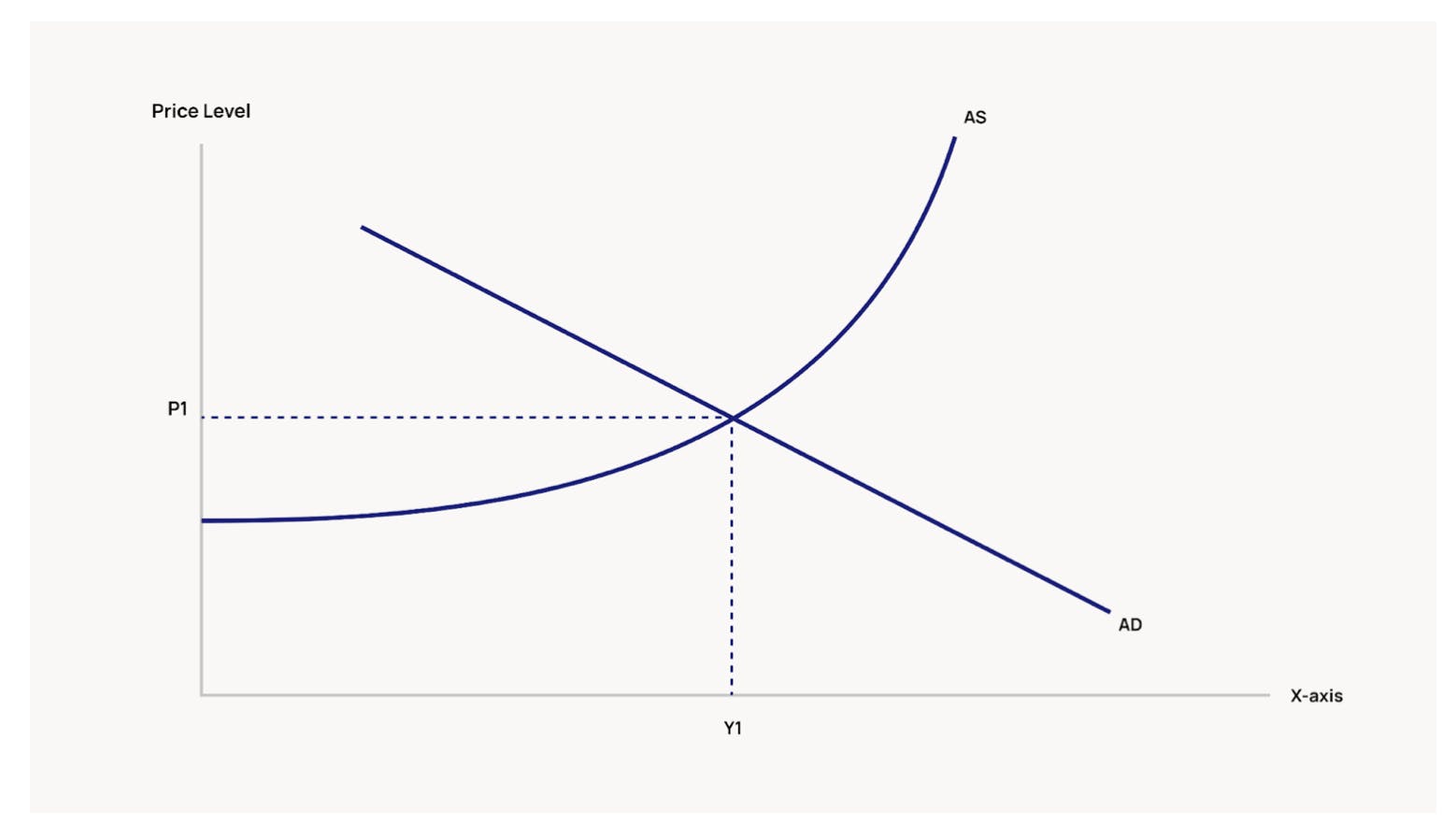
In the AD-AS model, the level of prices in the economy is shown on the vertical (Y) axis and real GDP, GDP adjusted for inflation, on the horizontal (X) axis. The X-axis is also commonly labelled as output or national income. A standard classical representation of the model consists of three curves: aggregate demand, short-run aggregate supply, and long-run aggregate supply, as in Figure 1 below.

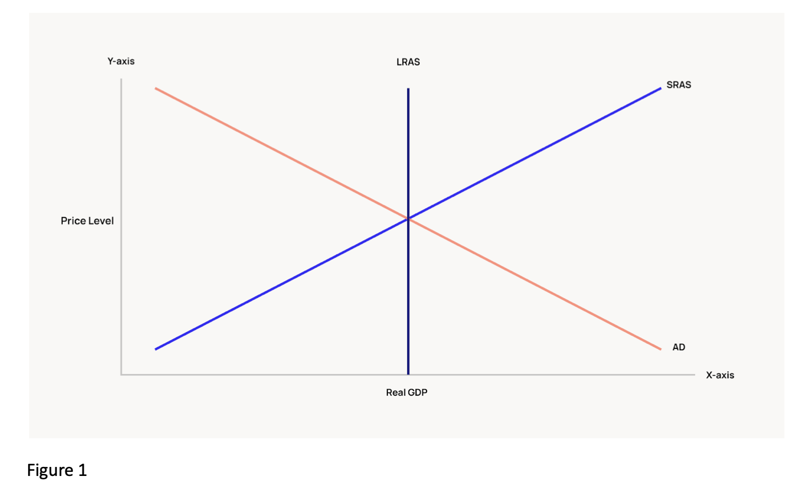
Explaining the 3 AD-AS Model curves

Let’s look at those curves and their determinants in more detail.

Aggregate demand curve

This is a representation of the total demand for goods and services produced domestically in an economy over a set period of time. The determinants of the curve and the reason for its downward slope can be expressed as AD = C + I + G + (X - M), which means AD is the sum of consumer expenditure (C), investment (I), government spending (G), and exports (X) minus imports (M). It shows the inverse relationship between price levels and real GDP or output. For example, a fall in the price level will likely lead to an increase in consumer expenditure as consumers’ purchasing power increases (assuming wages remain constant), which in turn increases demand for output. Lower prices can also increase demand for exports, as exports become cheaper, which raises GDP. Finally, lower prices often mean lower interest rates, which also stimulates an increase in spending and investment. These effects are called the wealth effect, the net export effect, and the interest rate effect. 

Short-run aggregate supply (SRAS) curve

This is a representation of the total supply of goods and services produced domestically in an economy over a certain period of time. You will notice that we differentiate between the short-run and the long-run AS curves. In the short-run, the AS curve slopes upwards, indicating that as prices increase firms will supply more and output will increase. This is because the SRAS curve is primarily determined by the costs of production in relation to the prices of products. It is assumed that in the short-run, the main costs of production, particularly wages, are “sticky”, meaning that they do not react quickly to changes in the price level. Therefore, if prices go up, while other costs remain stable, firms will be incentivised to produce more at the new price level in order to earn more profits, thereby increasing output. 

Long-run aggregate supply (LRAS) curve

According to classical economists, in the long-run, the AS curve is vertical. This is because price levels do not affect long-run supply. It is assumed that the only factors affecting long-run output will be determinants of the size of the economy, namely labour, capital, natural resources, and technological capabilities. Therefore, output will be the same at any price level as the costs of production will have had time to fully adjust to new price levels, i.e. there is no “stickiness”. 

Shifts in Aggregate Demand

In Demystifying Global Macroeconomics, John Marthinsen explains that,

In the section above, we explained what causes movements along the curves, namely changes in price level, shown on the AD curve in Figure 2 below. Price level, as a variable, is endogenous to or dependent on the model. However, what many are interested in is how to shift the curves outwards or inwards. Shifts in the AD curve are shown in Figure 3 below. Shifts are caused by exogenous variables or variables external to the model.

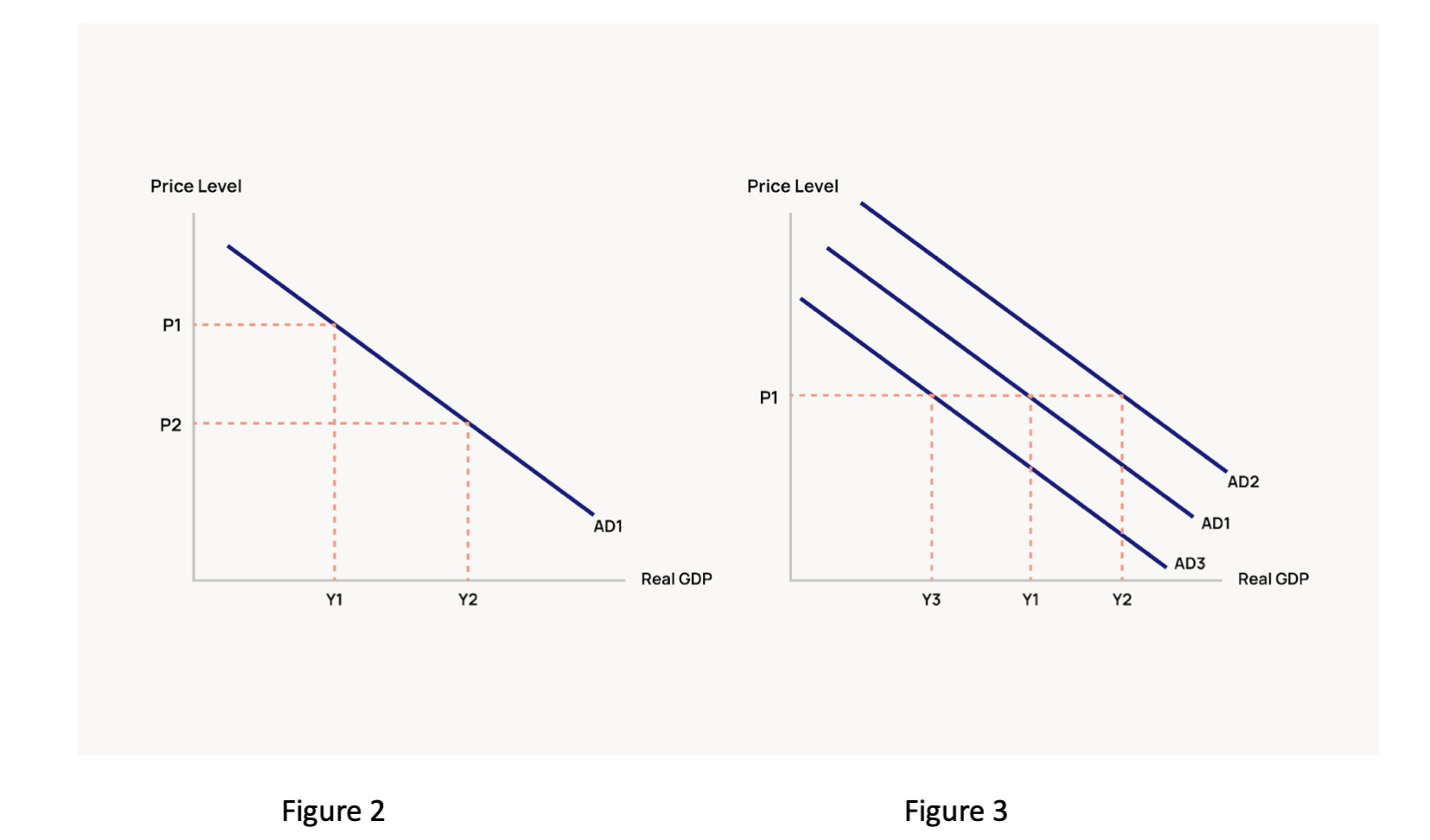
The AD curve shifts outwards or, indeed, retracts inwards, when there are changes in its underlying components, namely consumption, investment, government spending, or net exports (exports minus imports). There are multiple variables that could affect AD, here are just a few:

• Taxation: tax cuts could increase consumer’s disposable income and therefore increase consumption. Tax rises would have the opposite effect.
• Interest rates: a rise in interest rates could increase consumer’s propensity to save rather than consume, this would also increase the cost of investment, which would likely lead to less investment. 
• Wealth levels: a stock market crash or a housing market crash would decrease consumer’s wealth and therefore consumption. 
• Consumer or business confidence: high inflation can have a significant negative effect on consumer and business confidence, reducing propensity to spend and invest.
• Exchange rates: a strong domestic currency relative to other currencies may stimulate imports and reduce exports as imports become cheaper and exports more expensive (assuming the price elasticity of imports and exports is high, i.e., sensitive to changes in price).
  

Aggregate Supply in the Short- and Long-run

Both the short- and long-run AS curves can shift either to the right or left, Figures 4 and 5 below. Shifts in the SRAS curve are mostly caused by factors influencing firms’ decisions on how much to produce, for example a change in the costs of production, particularly wages, changes in business confidence, changes to business taxes, government regulation changes, etc. For example, strike action that leads to a rise in wages (all other things remaining equal), may lead to a reduction in output. These types of supply shocks may well lead to a decrease in output, but are commonly passed onto consumers to some extent in the form of higher prices.

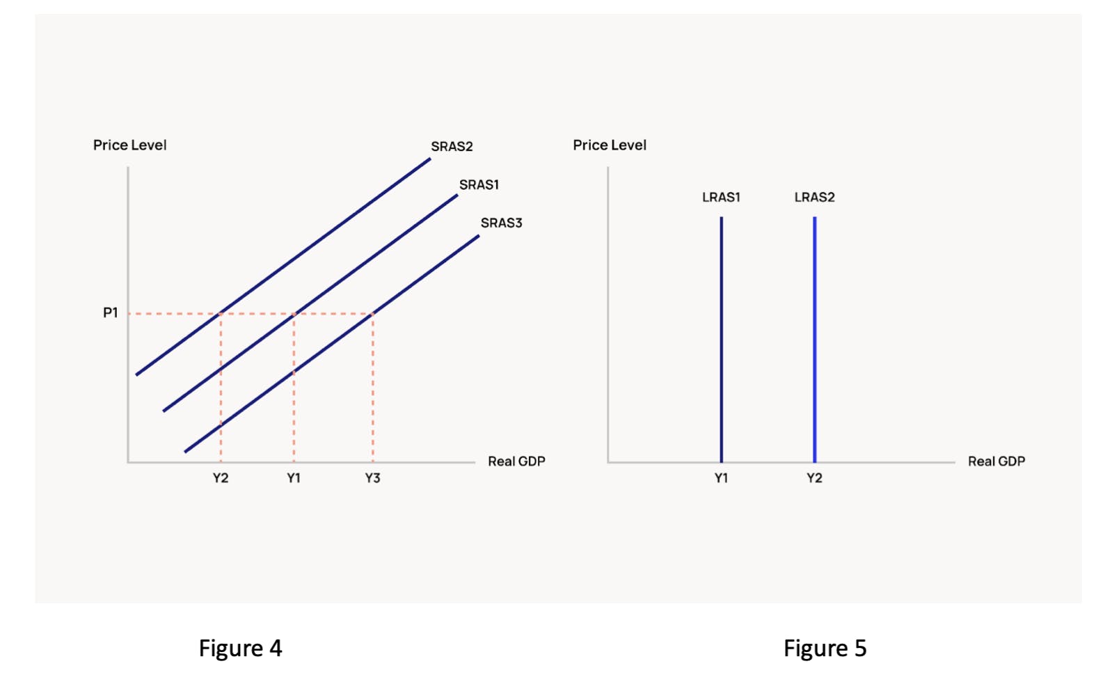
The long-run aggregate supply curve (LRAS) is fixed at the economy’s natural level of output, which refers to the total output of an economy when all its resources are fully employed, including labour. In reality, full employment is a rare occurrence, but is a useful tool enabling analysis of the potential output of the economy against real output. The natural level of output could be affected by an increase in the size of the labour force, through a change in immigration policy allowing more foreign workers in, for example. This would be represented by a shift of the LRAS curve to the right. Other factors affecting natural levels of output could be the availability of resources or the productivity of its workforce. For example, if a country discovers untapped natural resources or acquires new technology that increases worker productivity, this could all increase potential output. 

Finding Equilibrium

Naturally, it is rare for factors that change AS or AD to occur in isolation. We need to analyse the interaction between AD and AS through changes in the point of equilibrium. The short-run equilibrium point is where the AD curve intersects with the SRAS curve and shows the level of prices and output in the economy at the current moment. Policy makers and central banks compare this to the point of long-run equilibrium, or where the AD curve intersects with the SRAS and LRAS curves.

This tool is used by governments and central banks to estimate the current state of the economy or the point we are at in the business cycle. Kevin Hoover puts it very succinctly in his comprehensive book on Applied Intermediate Macroeconomics, “the plans of aggregate suppliers and aggregate demanders are not automatically coordinated…The substance of macroeconomics concerns the problem of coordinating those plans.” (2011)

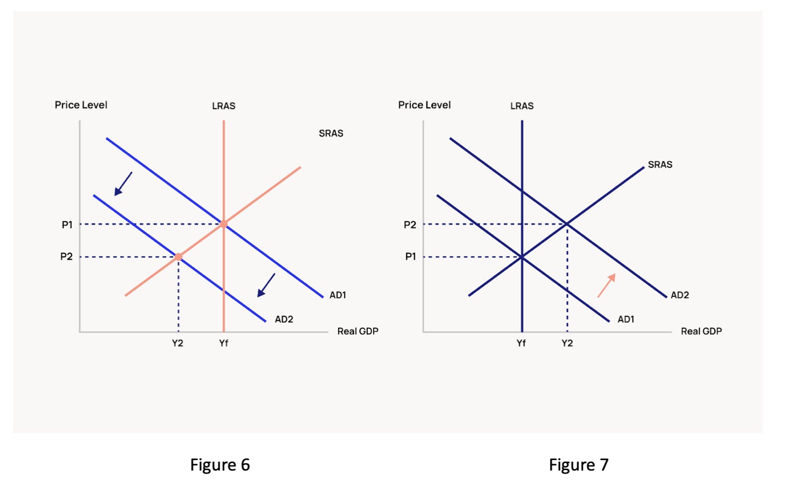
For example, in Figure 6, we see a situation in which the short-run equilibrium has shifted to the left of the long-run equilibrium. This is called a recessionary gap or a negative output gap, where output is less than the potential output of the economy. This could happen when a demand or supply shock causes output to drop. A negative output gap is typically caused by weak demand in the economy, leading to rising unemployment and deflation. 

In Figure 7, we see a positive output gap or inflationary gap, where the short-run equilibrium has shifted to the right. This is perhaps harder to imagine, how can we produce more than the potential output of the economy? A good example of this is working overtime. During an economic boom, AD can outstrip the point at which the economy is fully employing its resources (the LRAS curve), meaning firms need to pay overtime and workers will be asked to work extra hours to meet the demand. In this scenario, labour is working at a level over and above full employment and there is likely to be inflationary pressure on the economy. This is unsustainable over the long-term, firms will need to hire more workers to meet the demand, therefore, the LRAS curve will shift to the right and a new equilibrium will be found. 

In both cases, if these shifts are believed to be significant and sustained, governments will most likely be debating what they can do to close the output gap and help return the economy to equilibrium. Think of the recent COVID-19 epidemic, an excellent example of both demand and supply shocks acting on the global economy. In many economies around the world, the pandemic led to a sharp drop in output. Demand slumped as consumers were not allowed to leave their homes, uncertainty led consumers and investors to put off purchasing and investment decisions. Supply was also disrupted as workers could not come into work and global supply chains fell apart. In the UK, GDP fell 21.4% in the second quarter of 2020 compared to the average for 2019. This led to a policy response from the UK government, with massive increases in government spending to mitigate the worst of the downward pressure. 

Aggregate Supply or Aggregate Demand: The Big Debate

Was the government right to do this? The AD-AS model touches on one of the biggest debates in economics. To increase real GDP and raise living standards, should there be a strong government intervention? And if so, should they focus on increasing aggregate demand or aggregate supply? Which is the driver of economic output and which can help you when your country is heading for a recession? 

The Great Depression of the 1930s turned economic thinking on its head. Up to that point, classical economics or supply-side economics had reigned mostly due to the work of Jean-Baptiste Say. In his work, A Treatise on Political Economy, (1803 [2017]) he argues that supply precedes demand as to have demand a consumer must have first produced and earned money from that production in order to then consume other things.  This came to be known as Say’s Law.

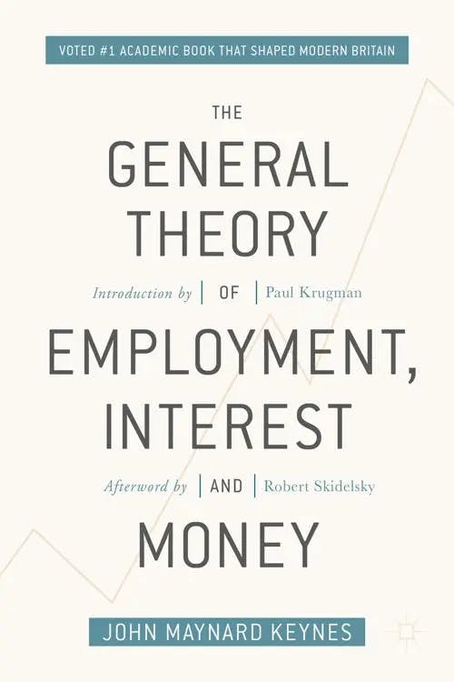
In 1936, John Maynard Keynes, one of the most important people in modern economics, published The General Theory of Employment, Interest, and Money (1936 [2018]) as a counter to Say’s Law. He chastised earlier economists for:

Keynes believed that governments could reduce unemployment and increase GDP by stimulating demand as opposed to supply. 

It is important to note that he also disagrees with the classical representation of the AD-AS model (shown above), believing that rather than a SRAS and vertical LRAS, there is only one AS curve, which starts out horizontal and becomes vertical as output increases. This is to do with the elasticity of aggregate supply. A representation of the Keynesian AD-AS model is below and it is worth being familiar with both.

The debate over the relative importance of AD as opposed to AS continues to this day and signifies the complexity of the national economy and responses to economic shocks. Nevertheless, the AD-AS model is worth understanding thoroughly as it remains a key tool for economists today in helping to make important policy decisions.

Further Macroeconomics reading on Perlego

Economics: A Complete Introduction

A Concise Guide to Macroeconomics

Principles of Macroeconomics

Macroeconomics in Context

Macroeconomics: Principles & Policy

Macroeconomics for Dummies